Fast word2vec

Fast word2vec

지난 POST에서 word2vec 의 종류중 하나인 CBOW를 살펴보게 되면 아래 그림과 같다.

위의 그림의 구조는 큰 2가지 문제점을 가지고 있다.
예를들어 어휘수가 위의 그림과 같이 100만개라고 한다면 다음의 과정에서 상당한 메모리와 계산량이 필요하다.

• 입력층의 원핫 표현과 가중치 행렬 \(W_{in}\)의 곱 계산
• 은닉층과 가중치 행렬 \(W_{out}\)의 곱 및 Softmax 계층의 계산

아래 과정은 각각의 문제점에 대한 해결방안 제시이다.

Embedding 계층

위의 두 문제점 중 먼저 입력층의 원핫 표현과 가중치 행렬 \(W_{in}\)의 곱 계산을 해결하기 위한 Embedding 계층에 대해서 알아보자
위의 문제를 해결하기 위하여 새로운 Embedding이라는 계층을 추가하였다.
먼저 Embedding이라는 개념을 알아보면 다음과 같다.
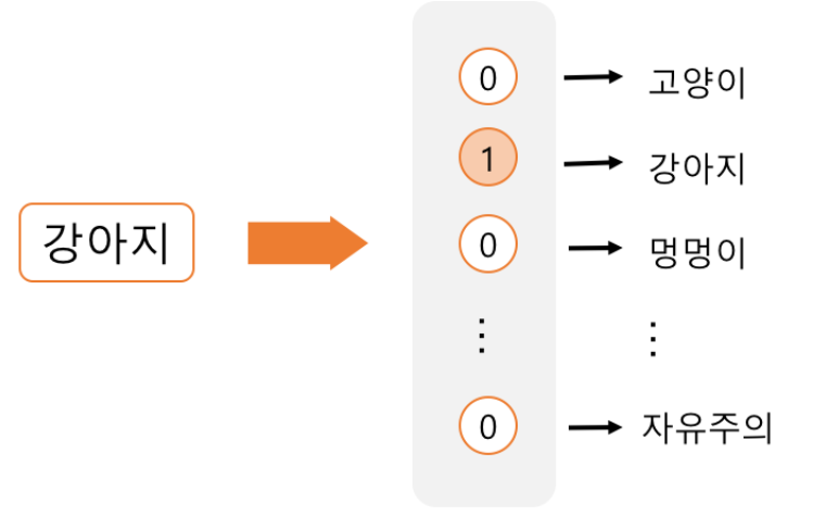
Embedding이란 Machine Learning Algorithm에서 자연어 처리 문제를 다룰 떄 널리 사용되는 기법이다. 이전 까지 사용하였던 방법은 One-hot-Encoding 이다.
One-hot-Encoding이란 단어 집합의 크기를 벡터의 차원으로 하고, 표현하고 싶은 단어의 인덱스에 1의 값을 부여하고, 다른 인덱스에는 0을 부여하는 단어의 벡터 표현 방식이다.
이러한 방식은 크게 2가지의 단점이 생기게 된다.

1. 단어의 개수가 늘어날 수록, 벡터를 저장하기 위해 필요한 공간이 계속 늘어난다.
2. 단어의 유사성을 전혀 표현하지 못한다.

이러한 One-hot-Encoding은 하나의 원소만 1이고 나머지의 원소는 0이므로 Sparse하다고 표현된다.

이러한 Sparse한 표현 형태를 Dense한 임베딩 행렬을 곱해서 아래와 같이 나타낼 수 있다.

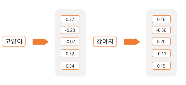
이러한 Dense한 Embedding은 다음과 같은 3가지의 장점을 가지게 된다.

1. 데이터의 표현 형태를 Sparse한 형태에서 Dense한 형태로 바꿔서더욱 효율적인 학습이 가능하도록 만들어 준다.
2. 데이터의 차원을 축소해서 연산량을 감소시킨다.
3. 단어 사이의 유사성을 표현할 수 있다.

위에서 설명한 Embedding 계층에 대한 Model은 아래 그림과 같다.

즉 저번 Post에서 설명한 W는 각 행이 각 단어의 분산 표현에 해당한다. 와 Input Data의 One-Hot-Encoding을 생각하여 Input Data를 W의 해당 단어의 분산 표현으로서 나타낸다는 의미이다.
위의 특징을 합쳐서 Embedding 계층의 Forward는 결과적으로 단지 행렬(W)의 특정 행을 추출하는 방식으로 구현할 수 있다.
위와 같은 Forward를 구성하였으므로 BackWard의 경우에도 해당하는 특정 행에만 기울기를 전달하고 나머지는 0으로서 구현하면 된다.
여기서 Batch 처리를 생각하게 되면 Backward의 경우 같은 Index가 오는 경우에 값이 덮여씌워지는 현상이 발생할 수 있기때문에 더하기 연산으로 구현해야 한다.
이러한 Embedding 계층은 아래와 같이 구현될 수 있다.

class Embedding:
    def __init__(self, W):
        self.params = [W]
        self.grads = [np.zeros_like(W)]
        self.idx = None

    def forward(self, idx):
        W, = self.params
        self.idx = idx
        #matmul연산 없이 W의 해당 index만 추출
        out = W[idx]
        return out

    def backward(self, dout):
        dW, = self.grads
        dW[...] = 0
        #덮어 씌위는 것이 아닌 더하기 로서 같은 idx올 경우 생각
        np.add.at(dW, self.idx, dout)
        return None

네거티브 샘플링

위의 두 문제점 중 은닉층과 가중치 행렬 \(W_{out}\)의 곱 및 Softmax 계층의 계산을 해결하기 위한 네거티브 샘플링에 대해서 알아보자

네거티브 샘플링의 핵심 아이디어는 다중분류를 이진분류로 근사화 하는 것 이다.
즉 연산이 오래걸리는 Softmax의 계산을 단순한 Sigmoid계산으로서 해결하자는 것 이다.

네거티브 샘플링은 아래 그림과 같다.

다중분류를 이진분류로 바뀌게 되면 다음과 같은 문제점이 발생하게 된다.
다중분류는 you 와 goodbye가 주어지면 정답인 say를 높히는 방향으로 진행되었다.
이러한 다중분류가 이진분류로서 you 와 goodbye가 주어지면 say가 정답입니까? Yes/No로서 신경망을 구축해야 한다.

Forward
먼저 \(W_{out}\)의 곱 계산을 어떻게 해결할 것인지를 생각해 보자.
전체적인 아이디어는 위에서의 Embedding과 같다.
저번 Post에서 설명한 U는 W와 마찬가지로 각 행이 각 단어의 분산 표현에 해당한다. Embedding과 마찬가지로 곱 계산을 하는 것이 아닌 해당하는 행을 그저 가져오면 된다는 의미이다.
이렇게 가져온 행과 은닉층의 뉴런과의 내적으로 인하여 \(W_{out}\)의 곱 계산을 어떻게 해결할 수 있다.

class EmbeddingDot:
    def __init__(self, W):
        self.embed = Embedding(W)
        self.params = self.embed.params
        self.grads = self.embed.grads
        self.cache = None

    def forward(self, h, idx):
        target_W = self.embed.forward(idx)
        out = np.sum(target_W * h, axis=1)

        self.cache = (h, target_W)
        return out

    def backward(self, dout):
        h, target_W = self.cache
        dout = dout.reshape(dout.shape[0], 1)

        dtarget_W = dout * h
        self.embed.backward(dtarget_W)
        dh = dout * target_W
        return dh

이러한 결과로 인한 하나의 뉴런이 Output으로 나오기 때문에 Softmax 계층의 계산을 Sigmoid로서 단순한 계산으로서 바꿀 수 있다.

Backward
실질적인 Parameter를 사용하기 위해 LossFunction을 미분할 줄 알아야 한다.
Loss Function을 CrossEntropy를 사용하고 Activation Function은 Sigmoid가 된다.
Loss Function을 미분하는 과정은 아래와 같다.

$$y = \frac{1}{1+ exp(-x)}$$

$$\frac{\partial{y}}{\partial{x}} = y(1-y)$$

$$L = -(tlogy + (1-t)log(1-y))$$

$$\frac{\partial{L}}{\partial{x}} = -\frac{\partial{tlogy}}{\partial{x}} + \frac{\partial{tlog(1-t)log(1-y)}}{\partial{x}}$$

$$ = -t\frac{1}{y}y(1-y) + (1-t)\frac{1}{1-y}y(1-y)$$

$$= -t(1-y) + (1-t)y$$

$$= y-t$$

위의 과정만으로 Loss를 측정해서 학습을 진행할 경우 Sigmoid의 Parameter라 긍정적인 예인 “say”에 대해서만 학습하게 된다.

정확한 분류를 위해서는 긍정적인인 예 “say”에 대해서는 출력을 1에 가깝게 만들고 “say”외의 모든 단어에 대해서는 0 으로서 출력값이 나오게 학습을 하는것이 목표이다.

모든 부정적 예를 대상으로 이진 분류를 학습시키게 되면 연산량이 많아지므로 일부 부정적인 예를 통하여 학습하는 것이 원래 목표였던 연산량을 줄이는 것에대한 적합한 방향이다.
이러한 적은 수의 분정적 예를 샘플링해 사용하는 것이 네거티브 샘플링 기법이다.
최종적인 Loss는 이러한 정답인 Loss와 네거티브 Loss의 합이 된다.
위와 같이 Sigmoid with Loss 계층은 다음과 같이 구현 될 수 있다.

def cross_entropy_error(y, t):
    if y.ndim == 1:
        t = t.reshape(1, t.size)
        y = y.reshape(1, y.size)
        
    # 정답 데이터가 원핫 벡터일 경우 정답 레이블 인덱스로 변환
    if t.size == y.size:
        t = t.argmax(axis=1)
             
    batch_size = y.shape[0]

    return -np.sum(np.log(y[np.arange(batch_size), t] + 1e-7)) / batch_size

class SigmoidWithLoss:
    def __init__(self):
        self.params, self.grads = [], []
        self.loss = None
        self.y = None  #  # sigmoid의 출력
        self.t = None  # 정답 데이터

    def forward(self, x, t):
        self.t = t
        self.y = 1 / (1 + np.exp(-x))

        self.loss = cross_entropy_error(np.c_[1 - self.y, self.y], self.t)

        return self.loss

    def backward(self, dout=1):
        batch_size = self.t.shape[0]

        dx = (self.y - self.t) * dout / batch_size
        return dx

네거티브 샘플링의 샘플링 기법
네거티브 샘플링을 어떻게 샘플링을 할 것인지도 하나의 문제이다.
자주 등장하는 단어를 많이 추출하고 드물게 등장하는 단어를 적게 추출하는 것이 Model의 성능을 좋게 만들 것이라는 것을 알 수 있다.(희소한 단어 자체는 나올 확률이 매우 적기 때문)
이러한 과정은 각 확률에 대해 0.75를 곱함으로 인하여 출현확률이 낮은 확률은 올리고 너무 높은 확률은 낮추는 방향으로 진행하여 출현확률이 낮은 단어를 버리지 않는 방식으로 진행한다.
UnigramSampler

• corpus: 말뭉치
• power: 각 확률에 곱할 인수
• sample_size: 샘플링을 수행할 횟수

np.random.choice(words,size,replace,p)

• words: 랜덤하게 뽑을 집합
• size: 샘플링할 size
• replace: False시 반복 X
• p: 각가의 Sampling될 확률

네거티브 샘플링의 샘플링 기법

class UnigramSampler:
    def __init__(self, corpus, power, sample_size):
        self.sample_size = sample_size
        self.vocab_size = None
        self.word_p = None

        counts = collections.Counter()
        for word_id in corpus:
            counts[word_id] += 1

        vocab_size = len(counts)
        self.vocab_size = vocab_size

        self.word_p = np.zeros(vocab_size)
        for i in range(vocab_size):
            self.word_p[i] = counts[i]

        self.word_p = np.power(self.word_p, power)
        self.word_p /= np.sum(self.word_p)

    def get_negative_sample(self, target):
        batch_size = target.shape[0]

        
        negative_sample = np.zeros((batch_size, self.sample_size), dtype=np.int32)

        for i in range(batch_size):
            p = self.word_p.copy()
            target_idx = target[i]
            p[target_idx] = 0
            p /= p.sum()
            negative_sample[i, :] = np.random.choice(self.vocab_size, size=self.sample_size, replace=False, p=p)
     
        
        return negative_sample

결과 확인

import numpy as np
import collections

corpus = np.array([0,1,2,3,4,1,2,3])
power = 0.75
sample_size = 2

sampler = UnigramSampler(corpus,power,sample_size)
target = np.array([1,3,0])
negative_sample = sampler.get_negative_sample(target)
print(negative_sample)

[[0 2]
 [1 4]
 [3 4]]

최종적인 네거티브 Sampling with Loss 계층을 구현한 Code이다.

아래 코드는 다음과 같은 과정으로 진행된 것이다.

1. 입력층의 원핫 표현과 가중치 행렬 W_in의 곱 계산을 해결하기 위한 Embedding 계층
2. W_out의 곱 계산 을 해결하기 위한 EmbeddingDot 계층(입력 Embedding + HiddenLayer Embedding)
3. BackPropagation을 위한 Sigmoid + CrossEntropy = Sigmoid With Loss 계층
4. 네거티브 샘플링의 샘플링을 위한 UnigramSampler
5. 네거티브 샘플링 계층 NegativeSampleingLoss(Embedding Dot + UnigramSample + Sigmoid With Loss)

class NegativeSamplingLoss:
    def __init__(self, W, corpus, power=0.75, sample_size=5):
        self.sample_size = sample_size
        self.sampler = UnigramSampler(corpus, power, sample_size)
        self.loss_layers = [SigmoidWithLoss() for _ in range(sample_size + 1)]
        self.embed_dot_layers = [EmbeddingDot(W) for _ in range(sample_size + 1)]

        self.params, self.grads = [], []
        for layer in self.embed_dot_layers:
            self.params += layer.params
            self.grads += layer.grads

    def forward(self, h, target):
        batch_size = target.shape[0]
        negative_sample = self.sampler.get_negative_sample(target)

        # 긍정적 예 순전파
        score = self.embed_dot_layers[0].forward(h, target)
        correct_label = np.ones(batch_size, dtype=np.int32)
        loss = self.loss_layers[0].forward(score, correct_label)

        # 부정적 예 순전파
        negative_label = np.zeros(batch_size, dtype=np.int32)
        for i in range(self.sample_size):
            negative_target = negative_sample[:, i]
            score = self.embed_dot_layers[1 + i].forward(h, negative_target)
            loss += self.loss_layers[1 + i].forward(score, negative_label)

        return loss

    def backward(self, dout=1):
        dh = 0
        for l0, l1 in zip(self.loss_layers, self.embed_dot_layers):
            dscore = l0.backward(dout)
            dh += l1.backward(dscore)

        return dh

CBOW Model

위의 최종적으로 얻은 네거티브 샘플링 계층을 활용하여 CBOW Model을 구현해보자.

class CBOW:
    def __init__(self, vocab_size, hidden_size, window_size, corpus):
        V, H = vocab_size, hidden_size

        # 가중치 초기화
        W_in = 0.01 * np.random.randn(V, H).astype('f')
        W_out = 0.01 * np.random.randn(V, H).astype('f')

        # 계층 생성
        self.in_layers = []
        for i in range(2 * window_size):
            layer = Embedding(W_in)  # Embedding 계층 사용
            self.in_layers.append(layer)
        self.ns_loss = NegativeSamplingLoss(W_out, corpus, power=0.75, sample_size=5)

        # 모든 가중치와 기울기를 배열에 모은다.
        layers = self.in_layers + [self.ns_loss]
        self.params, self.grads = [], []
        for layer in layers:
            self.params += layer.params
            self.grads += layer.grads

        # 인스턴스 변수에 단어의 분산 표현을 저장한다.
        self.word_vecs = W_in

    def forward(self, contexts, target):
        h = 0
        for i, layer in enumerate(self.in_layers):
            h += layer.forward(contexts[:, i])
        h *= 1 / len(self.in_layers)
        loss = self.ns_loss.forward(h, target)
        return loss

    def backward(self, dout=1):
        dout = self.ns_loss.backward(dout)
        dout *= 1 / len(self.in_layers)
        for layer in self.in_layers:
            layer.backward(dout)
        return None

Model Train

# 학습을 위한 함수
import numpy
import time
import matplotlib.pyplot as plt
from common import config
import pickle
from common.util import clip_grads
from common.trainer import Trainer
from common.optimizer import Adam
from common.util import create_contexts_target, to_cpu, to_gpu
from dataset import ptb
config.GPU=True

# 하이퍼 파라미터 설정
window_size = 5
hidden_size = 100
batch_size = 100
max_epoch = 10

# 데이터 읽기 + target, contexts 만들기
corpus, word_to_id, id_to_word = ptb.load_data('train')
vocab_size = len(word_to_id)

contexts, target = create_contexts_target(corpus, window_size)

# 모델 등 생성 - CBOW or SkipGram
model = CBOW(vocab_size, hidden_size, window_size, corpus)
# model = SkipGram(vocab_size, hidden_size, window_size, corpus)
optimizer = Adam()
trainer = Trainer(model,optimizer)

# 학습 시작
trainer.fit(contexts, target, max_epoch, batch_size, eval_interval = 3000) # eval_interval=500
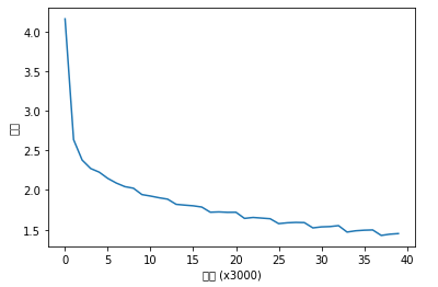
trainer.plot()

# 나중에 사용할 수 있도록 필요한 데이터 저장
word_vecs = model.word_vecs
if config.GPU:
    word_vecs = to_cpu(word_vecs)
params = {}
params['word_vecs'] = word_vecs.astype(np.float16)
params['word_to_id'] = word_to_id
params['id_to_word'] = id_to_word
pkl_file = 'cbow_params.pkl'  # or 'skipgram_params.pkl'
with open(pkl_file, 'wb') as f:
    pickle.dump(params, f, -1)

Model Train 결과

| 에폭 1 |  반복 1 / 9295 | 시간 0[s] | 손실 4.16
| 에폭 1 |  반복 3001 / 9295 | 시간 183[s] | 손실 2.64
| 에폭 1 |  반복 6001 / 9295 | 시간 404[s] | 손실 2.38
| 에폭 1 |  반복 9001 / 9295 | 시간 632[s] | 손실 2.27
| 에폭 2 |  반복 1 / 9295 | 시간 654[s] | 손실 2.23
| 에폭 2 |  반복 3001 / 9295 | 시간 880[s] | 손실 2.15
| 에폭 2 |  반복 6001 / 9295 | 시간 1086[s] | 손실 2.09
| 에폭 2 |  반복 9001 / 9295 | 시간 1273[s] | 손실 2.04
| 에폭 3 |  반복 1 / 9295 | 시간 1294[s] | 손실 2.02
| 에폭 3 |  반복 3001 / 9295 | 시간 1514[s] | 손실 1.94
| 에폭 3 |  반복 6001 / 9295 | 시간 1735[s] | 손실 1.92
| 에폭 3 |  반복 9001 / 9295 | 시간 1955[s] | 손실 1.90
| 에폭 4 |  반복 1 / 9295 | 시간 1977[s] | 손실 1.89
| 에폭 4 |  반복 3001 / 9295 | 시간 2196[s] | 손실 1.82
| 에폭 4 |  반복 6001 / 9295 | 시간 2414[s] | 손실 1.81
| 에폭 4 |  반복 9001 / 9295 | 시간 2631[s] | 손실 1.80
| 에폭 5 |  반복 1 / 9295 | 시간 2653[s] | 손실 1.79
| 에폭 5 |  반복 3001 / 9295 | 시간 2874[s] | 손실 1.72
| 에폭 5 |  반복 6001 / 9295 | 시간 3092[s] | 손실 1.72
| 에폭 5 |  반복 9001 / 9295 | 시간 3309[s] | 손실 1.72
| 에폭 6 |  반복 1 / 9295 | 시간 3330[s] | 손실 1.72
| 에폭 6 |  반복 3001 / 9295 | 시간 3549[s] | 손실 1.64
| 에폭 6 |  반복 6001 / 9295 | 시간 3770[s] | 손실 1.65
| 에폭 6 |  반복 9001 / 9295 | 시간 3985[s] | 손실 1.65
| 에폭 7 |  반복 1 / 9295 | 시간 4007[s] | 손실 1.64
| 에폭 7 |  반복 3001 / 9295 | 시간 4228[s] | 손실 1.58
| 에폭 7 |  반복 6001 / 9295 | 시간 4446[s] | 손실 1.59
| 에폭 7 |  반복 9001 / 9295 | 시간 4664[s] | 손실 1.59
| 에폭 8 |  반복 1 / 9295 | 시간 4685[s] | 손실 1.59
| 에폭 8 |  반복 3001 / 9295 | 시간 4906[s] | 손실 1.52
| 에폭 8 |  반복 6001 / 9295 | 시간 5126[s] | 손실 1.54
| 에폭 8 |  반복 9001 / 9295 | 시간 5346[s] | 손실 1.54
| 에폭 9 |  반복 1 / 9295 | 시간 5368[s] | 손실 1.55
| 에폭 9 |  반복 3001 / 9295 | 시간 5591[s] | 손실 1.47
| 에폭 9 |  반복 6001 / 9295 | 시간 5814[s] | 손실 1.49
| 에폭 9 |  반복 9001 / 9295 | 시간 6035[s] | 손실 1.49
| 에폭 10 |  반복 1 / 9295 | 시간 6057[s] | 손실 1.50
| 에폭 10 |  반복 3001 / 9295 | 시간 6278[s] | 손실 1.43
| 에폭 10 |  반복 6001 / 9295 | 시간 6499[s] | 손실 1.44
| 에폭 10 |  반복 9001 / 9295 | 시간 6719[s] | 손실 1.45

Model 평가

from common.util import most_similar, analogy

pkl_file = 'cbow_params.pkl'

with open(pkl_file, 'rb') as f:
    params = pickle.load(f)
    word_vecs = params['word_vecs']
    word_to_id = params['word_to_id']
    id_to_word = params['id_to_word']

# 가장 비슷한(most similar) 단어 뽑기
querys = ['you', 'year', 'car', 'toyota']
for query in querys:
    most_similar(query, word_to_id, id_to_word, word_vecs, top=5)

# 유추(analogy) 작업
print('-'*50)
analogy('king', 'man', 'queen',  word_to_id, id_to_word, word_vecs)
analogy('take', 'took', 'go',  word_to_id, id_to_word, word_vecs)
analogy('car', 'cars', 'child',  word_to_id, id_to_word, word_vecs)
analogy('good', 'better', 'bad',  word_to_id, id_to_word, word_vecs)

Model 평가 결과

[query] you
 we: 0.75439453125
 i: 0.70263671875
 your: 0.61083984375
 anything: 0.60498046875
 anybody: 0.6025390625

[query] year
 month: 0.86279296875
 week: 0.78125
 summer: 0.7744140625
 spring: 0.73291015625
 decade: 0.68310546875

[query] car
 truck: 0.62158203125
 window: 0.61328125
 cars: 0.5673828125
 auto: 0.55078125
 luxury: 0.5498046875

[query] toyota
 engines: 0.64501953125
 honda: 0.6103515625
 unocal: 0.60595703125
 ford: 0.60498046875
 seita: 0.60498046875
--------------------------------------------------

[analogy] king:man = queen:?
 woman: 5.5234375
 text: 5.01953125
 naczelnik: 4.7265625
 father: 4.671875
 a.m: 4.65625

[analogy] take:took = go:?
 came: 4.26171875
 began: 4.18359375
 went: 4.17578125
 're: 4.12109375
 eurodollars: 4.08984375

[analogy] car:cars = child:?
 a.m: 6.22265625
 rape: 5.60546875
 children: 5.5078125
 incest: 4.76171875
 woman: 4.62890625

[analogy] good:better = bad:?
 rather: 5.69140625
 more: 5.65625
 less: 5.27734375
 greater: 4.45703125
 faster: 3.873046875

---

참조: 원본코드
참조: taeu 블로그
참조: 밑바닥부터 시작하는 딥러닝2 코드에 문제가 있거나 궁금한 점이 있으면 wjddyd66@naver.com으로 Mail을 남겨주세요.