Ch5.SVM

Support Vector Machine

Classifiction Model중에서 많이 사용하는 Model중 하나이다.
SVM을 많이 사용하는 이유는 특히, Kernel Trick이라는 기법을 사용하여 Linear뿐만 아니라 Non-Linear한 Decision Boundary를 만들 수 있기 때문이다.

SVM의 자세한 내용의 링크는 다음과 같다.

• Linear Support Vector Machine
• Non Linear Support Vector Machine

Setup

실제 Project를 진행하기 앞서 사용하고자 하는 Library확인 및 원하는 Version(Python 언어 특성상 Version에 많이 의존하게 된다.)이 설치되어있는지 확인하는 작업이다.
또한, 자주 사용하게 될 Function이나, Directory를 지정하기도 한다.

# Python ≥3.5 is required
import sys
assert sys.version_info >= (3, 5)

# Scikit-Learn ≥0.20 is required
import sklearn
assert sklearn.__version__ >= "0.20"

# Common imports
import numpy as np
import os

# to make this notebook's output stable across runs
np.random.seed(42)

# To plot pretty figures
%matplotlib inline
import matplotlib as mpl
import matplotlib.pyplot as plt
mpl.rc('axes', labelsize=14)
mpl.rc('xtick', labelsize=12)
mpl.rc('ytick', labelsize=12)

# Where to save the figures
PROJECT_ROOT_DIR = "."
CHAPTER_ID = "svm"
IMAGES_PATH = os.path.join(PROJECT_ROOT_DIR, "images", CHAPTER_ID)
os.makedirs(IMAGES_PATH, exist_ok=True)

def save_fig(fig_id, tight_layout=True, fig_extension="png", resolution=300):
    path = os.path.join(IMAGES_PATH, fig_id + "." + fig_extension)
    print("Saving figure", fig_id)
    if tight_layout:
        plt.tight_layout()
    plt.savefig(path, format=fig_extension, dpi=resolution)

Linear Support Vector Machine

SVM의 종류중 Linear하게 Decision Boundary를 정의하는 방법이다.

Hard Margin SVM

Distance가 가장 가까운 서로 다른 Class의 Distance가 가장 멀어지도록 Dicision boundary를 설정하는 방법이다.

from sklearn.svm import SVC
from sklearn import datasets

iris = datasets.load_iris()
X = iris["data"][:, (2, 3)]  # petal length, petal width
y = iris["target"]

setosa_or_versicolor = (y == 0) | (y == 1)
X = X[setosa_or_versicolor]
y = y[setosa_or_versicolor]

# SVM Classifier model
svm_clf = SVC(kernel="linear", C=float("inf"))
svm_clf.fit(X, y)

# Bad models
x0 = np.linspace(0, 5.5, 200)
pred_1 = 5*x0 - 20
pred_2 = x0 - 1.8
pred_3 = 0.1 * x0 + 0.5

def plot_svc_decision_boundary(svm_clf, xmin, xmax):
    w = svm_clf.coef_[0]
    b = svm_clf.intercept_[0]

    # At the decision boundary, w0*x0 + w1*x1 + b = 0
    # => x1 = -w0/w1 * x0 - b/w1
    x0 = np.linspace(xmin, xmax, 200)
    decision_boundary = -w[0]/w[1] * x0 - b/w[1]

    margin = 1/w[1]
    gutter_up = decision_boundary + margin
    gutter_down = decision_boundary - margin

    svs = svm_clf.support_vectors_
    plt.scatter(svs[:, 0], svs[:, 1], s=180, facecolors='#FFAAAA')
    plt.plot(x0, decision_boundary, "k-", linewidth=2)
    plt.plot(x0, gutter_up, "k--", linewidth=2)
    plt.plot(x0, gutter_down, "k--", linewidth=2)

fig, axes = plt.subplots(ncols=2, figsize=(10,2.7), sharey=True)

plt.sca(axes[0])
plt.plot(x0, pred_1, "g--", linewidth=2)
plt.plot(x0, pred_2, "m-", linewidth=2)
plt.plot(x0, pred_3, "r-", linewidth=2)
plt.plot(X[:, 0][y==1], X[:, 1][y==1], "bs", label="Iris versicolor")
plt.plot(X[:, 0][y==0], X[:, 1][y==0], "yo", label="Iris setosa")
plt.xlabel("Petal length", fontsize=14)
plt.ylabel("Petal width", fontsize=14)
plt.legend(loc="upper left", fontsize=14)
plt.axis([0, 5.5, 0, 2])

plt.sca(axes[1])
plot_svc_decision_boundary(svm_clf, 0, 5.5)
plt.plot(X[:, 0][y==1], X[:, 1][y==1], "bs")
plt.plot(X[:, 0][y==0], X[:, 1][y==0], "yo")
plt.xlabel("Petal length", fontsize=14)
plt.axis([0, 5.5, 0, 2])

save_fig("large_margin_classification_plot")
plt.show()

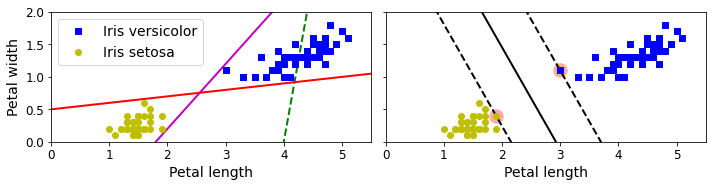
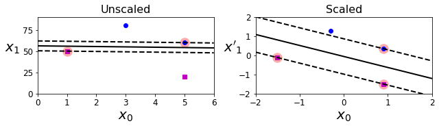
이러한 SVM은 서로다른 Class의 Dataset의 거리를 최대화 하는 것 이므로 Dataset을 Scaling하는 것이 Model의 성능이 좋아진다.

Xs = np.array([[1, 50], [5, 20], [3, 80], [5, 60]]).astype(np.float64)
ys = np.array([0, 0, 1, 1])
svm_clf = SVC(kernel="linear", C=100)
svm_clf.fit(Xs, ys)

plt.figure(figsize=(9,2.7))
plt.subplot(121)
plt.plot(Xs[:, 0][ys==1], Xs[:, 1][ys==1], "bo")
plt.plot(Xs[:, 0][ys==0], Xs[:, 1][ys==0], "ms")
plot_svc_decision_boundary(svm_clf, 0, 6)
plt.xlabel("$x_0$", fontsize=20)
plt.ylabel("$x_1$    ", fontsize=20, rotation=0)
plt.title("Unscaled", fontsize=16)
plt.axis([0, 6, 0, 90])

from sklearn.preprocessing import StandardScaler
scaler = StandardScaler()
X_scaled = scaler.fit_transform(Xs)
svm_clf.fit(X_scaled, ys)

plt.subplot(122)
plt.plot(X_scaled[:, 0][ys==1], X_scaled[:, 1][ys==1], "bo")
plt.plot(X_scaled[:, 0][ys==0], X_scaled[:, 1][ys==0], "ms")
plot_svc_decision_boundary(svm_clf, -2, 2)
plt.xlabel("$x_0$", fontsize=20)
plt.ylabel("$x'_1$  ", fontsize=20, rotation=0)
plt.title("Scaled", fontsize=16)
plt.axis([-2, 2, -2, 2])

save_fig("sensitivity_to_feature_scales_plot")

또한, Hard Margin SVM은 Outlier에 민감하다. 이러한 Outlier에 의하여 Hard Margin SVM을 사용하거나, 사용할 수 없는 것을 확인할 수 있다.

X_outliers = np.array([[3.4, 1.3], [3.2, 0.8]])
y_outliers = np.array([0, 0])
Xo1 = np.concatenate([X, X_outliers[:1]], axis=0)
yo1 = np.concatenate([y, y_outliers[:1]], axis=0)
Xo2 = np.concatenate([X, X_outliers[1:]], axis=0)
yo2 = np.concatenate([y, y_outliers[1:]], axis=0)

svm_clf2 = SVC(kernel="linear", C=10**9)
svm_clf2.fit(Xo2, yo2)

fig, axes = plt.subplots(ncols=2, figsize=(10,2.7), sharey=True)

plt.sca(axes[0])
plt.plot(Xo1[:, 0][yo1==1], Xo1[:, 1][yo1==1], "bs")
plt.plot(Xo1[:, 0][yo1==0], Xo1[:, 1][yo1==0], "yo")
plt.text(0.3, 1.0, "Impossible!", fontsize=24, color="red")
plt.xlabel("Petal length", fontsize=14)
plt.ylabel("Petal width", fontsize=14)
plt.annotate("Outlier",
             xy=(X_outliers[0][0], X_outliers[0][1]),
             xytext=(2.5, 1.7),
             ha="center",
             arrowprops=dict(facecolor='black', shrink=0.1),
             fontsize=16,
            )
plt.axis([0, 5.5, 0, 2])

plt.sca(axes[1])
plt.plot(Xo2[:, 0][yo2==1], Xo2[:, 1][yo2==1], "bs")
plt.plot(Xo2[:, 0][yo2==0], Xo2[:, 1][yo2==0], "yo")
plot_svc_decision_boundary(svm_clf2, 0, 5.5)
plt.xlabel("Petal length", fontsize=14)
plt.annotate("Outlier",
             xy=(X_outliers[1][0], X_outliers[1][1]),
             xytext=(3.2, 0.08),
             ha="center",
             arrowprops=dict(facecolor='black', shrink=0.1),
             fontsize=16,
            )
plt.axis([0, 5.5, 0, 2])

save_fig("sensitivity_to_outliers_plot")
plt.show()

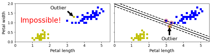
이러한 Hard Margin SVM의 해결방법으로는 다음과 같은 2가지 방법이 있다.

1. Outlier를 인정하고 Penalty를 적용한다. => Soft Margin SVM
2. Kernel Trick으로서 다차원(Linear Regression에서 Polynomial)으로서 Data를 옮겨서 SVM을 적용한다. => Non Linear Support Vector Machine

Soft Margin SVM

Hard Margin SVM의 해결 방법으로서 Penalty를 적용하는 방법이다.
Penalty의 종류로서는 크게 Hinge Loss, Zero-one Loss가 적용된다.

위의 링크에서 설명한 것과 같이 이러한 Hinge Loss는 Penalty의 크기를 C로서 지정할 수 있다.

import numpy as np
from sklearn import datasets
from sklearn.pipeline import Pipeline
from sklearn.preprocessing import StandardScaler
from sklearn.svm import LinearSVC

iris = datasets.load_iris()
X = iris["data"][:, (2, 3)]  # petal length, petal width
y = (iris["target"] == 2).astype(np.float64)  # Iris virginica

scaler = StandardScaler()
svm_clf1 = LinearSVC(C=1, loss="hinge", random_state=42)
svm_clf2 = LinearSVC(C=100, loss="hinge", random_state=42)

scaled_svm_clf1 = Pipeline([
        ("scaler", scaler),
        ("linear_svc", svm_clf1),
    ])
scaled_svm_clf2 = Pipeline([
        ("scaler", scaler),
        ("linear_svc", svm_clf2),
    ])

scaled_svm_clf1.fit(X, y)
scaled_svm_clf2.fit(X, y)

# Convert to unscaled parameters
b1 = svm_clf1.decision_function([-scaler.mean_ / scaler.scale_])
b2 = svm_clf2.decision_function([-scaler.mean_ / scaler.scale_])
w1 = svm_clf1.coef_[0] / scaler.scale_
w2 = svm_clf2.coef_[0] / scaler.scale_
svm_clf1.intercept_ = np.array([b1])
svm_clf2.intercept_ = np.array([b2])
svm_clf1.coef_ = np.array([w1])
svm_clf2.coef_ = np.array([w2])

# Find support vectors (LinearSVC does not do this automatically)
t = y * 2 - 1
support_vectors_idx1 = (t * (X.dot(w1) + b1) < 1).ravel()
support_vectors_idx2 = (t * (X.dot(w2) + b2) < 1).ravel()
svm_clf1.support_vectors_ = X[support_vectors_idx1]
svm_clf2.support_vectors_ = X[support_vectors_idx2]



fig, axes = plt.subplots(ncols=2, figsize=(10,2.7), sharey=True)

plt.sca(axes[0])
plt.plot(X[:, 0][y==1], X[:, 1][y==1], "g^", label="Iris virginica")
plt.plot(X[:, 0][y==0], X[:, 1][y==0], "bs", label="Iris versicolor")
plot_svc_decision_boundary(svm_clf1, 4, 5.9)
plt.xlabel("Petal length", fontsize=14)
plt.ylabel("Petal width", fontsize=14)
plt.legend(loc="upper left", fontsize=14)
plt.title("$C = {}$".format(svm_clf1.C), fontsize=16)
plt.axis([4, 5.9, 0.8, 2.8])

plt.sca(axes[1])
plt.plot(X[:, 0][y==1], X[:, 1][y==1], "g^")
plt.plot(X[:, 0][y==0], X[:, 1][y==0], "bs")
plot_svc_decision_boundary(svm_clf2, 4, 5.99)
plt.xlabel("Petal length", fontsize=14)
plt.title("$C = {}$".format(svm_clf2.C), fontsize=16)
plt.axis([4, 5.9, 0.8, 2.8])

save_fig("regularization_plot")

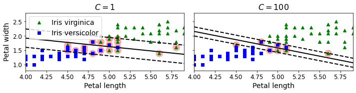
Data가 Linear하게 Classify되지 않는다고 가정하였을 경우, Penalty가 작으면 여전히 잘 분류하지 못하지만, 일정 크기 이상일 경우에는 어느정도의 Error를 감수하고 잘 분류하는 것을 살펴볼 수 있다. 이러한 C의 값은 무조건 크면 좋은 것이 아니라, 우리가 사용하고자 하는 Data의 신뢰도에 따라 Penalty를 줘야지 의미있는 Classification Model(SVM)을 설계할 수 있을 것 이다.

Non Linear Support Vector Machine

먼저 Dataset이 Dimension이 증가함에 따라서 어떻게 변하는지 살펴보면 다음과 같다.

X1D = np.linspace(-4, 4, 9).reshape(-1, 1)
X2D = np.c_[X1D, X1D**2]
y = np.array([0, 0, 1, 1, 1, 1, 1, 0, 0])

plt.figure(figsize=(10, 3))

plt.subplot(121)
plt.grid(True, which='both')
plt.axhline(y=0, color='k')
plt.plot(X1D[:, 0][y==0], np.zeros(4), "bs")
plt.plot(X1D[:, 0][y==1], np.zeros(5), "g^")
plt.gca().get_yaxis().set_ticks([])
plt.xlabel(r"$x_1$", fontsize=20)
plt.axis([-4.5, 4.5, -0.2, 0.2])

plt.subplot(122)
plt.grid(True, which='both')
plt.axhline(y=0, color='k')
plt.axvline(x=0, color='k')
plt.plot(X2D[:, 0][y==0], X2D[:, 1][y==0], "bs")
plt.plot(X2D[:, 0][y==1], X2D[:, 1][y==1], "g^")
plt.xlabel(r"$x_1$", fontsize=20)
plt.ylabel(r"$x_2$  ", fontsize=20, rotation=0)
plt.gca().get_yaxis().set_ticks([0, 4, 8, 12, 16])
plt.plot([-4.5, 4.5], [6.5, 6.5], "r--", linewidth=3)
plt.axis([-4.5, 4.5, -1, 17])

plt.subplots_adjust(right=1)

save_fig("higher_dimensions_plot", tight_layout=False)
plt.show()

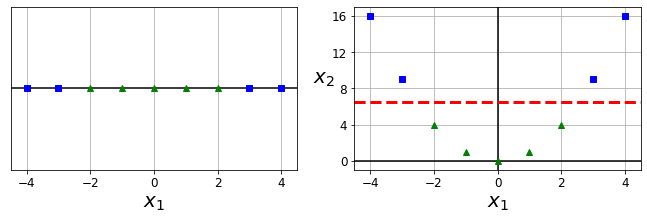
1 Dimension에서 직선으로 분류할 수 없었던 Dataset이 2차원으로서 변형되면서, 직선으로 분류될 수 있는 것을 살펴볼 수 있다.

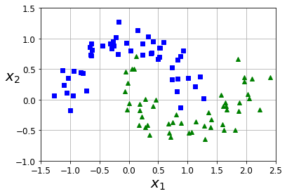
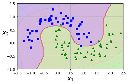
Kernel Trick을 사용하지는 않지만, Data의 Dimension을 늘리는 PolynomialFeatures를 사용하여 Model을 Fitting하면 다음과 같다. (Linear Regression -> Polynomial Regression이라고 생각하면 된다.)

from sklearn.datasets import make_moons
# Dataset
X, y = make_moons(n_samples=100, noise=0.15, random_state=42)

def plot_dataset(X, y, axes):
    plt.plot(X[:, 0][y==0], X[:, 1][y==0], "bs")
    plt.plot(X[:, 0][y==1], X[:, 1][y==1], "g^")
    plt.axis(axes)
    plt.grid(True, which='both')
    plt.xlabel(r"$x_1$", fontsize=20)
    plt.ylabel(r"$x_2$", fontsize=20, rotation=0)

plot_dataset(X, y, [-1.5, 2.5, -1, 1.5])
plt.show()

Polynomial Linear Support Vector Machine

from sklearn.datasets import make_moons
from sklearn.pipeline import Pipeline
from sklearn.preprocessing import PolynomialFeatures

polynomial_svm_clf = Pipeline([
        ("poly_features", PolynomialFeatures(degree=3)),
        ("scaler", StandardScaler()),
        ("svm_clf", LinearSVC(C=10, loss="hinge", random_state=42))
    ])

polynomial_svm_clf.fit(X, y)

def plot_predictions(clf, axes):
    x0s = np.linspace(axes[0], axes[1], 100)
    x1s = np.linspace(axes[2], axes[3], 100)
    x0, x1 = np.meshgrid(x0s, x1s)
    X = np.c_[x0.ravel(), x1.ravel()]
    y_pred = clf.predict(X).reshape(x0.shape)
    y_decision = clf.decision_function(X).reshape(x0.shape)
    plt.contourf(x0, x1, y_pred, cmap=plt.cm.brg, alpha=0.2)
    plt.contourf(x0, x1, y_decision, cmap=plt.cm.brg, alpha=0.1)

plot_predictions(polynomial_svm_clf, [-1.5, 2.5, -1, 1.5])
plot_dataset(X, y, [-1.5, 2.5, -1, 1.5])

save_fig("moons_polynomial_svc_plot")
plt.show()

Kernel Trick

실질적으로 Dataset의 Dimension을 높임으로 인하여 Non Linear한 Classification이 가능한 Support Vector Machine이다. Scikit Learn의 Argument는 다음과 같은 의미를 가지고 있다.

• degree: 몇차원의 Diemnsion으로 옮길 것 인가?
• coef0: 모델이 높은 차수와 낮은 차수에 얼마나 영향을 받을지 조절(이 부분은 잘 모르겠습니다. 아마 weight에 대한 Regularization으로 예측하고 있습니다.)
• C: Penalty의 Coefficient

또한, 많이 사용하는 Kernel은 다음과 같다.

$$K(x_i,x_j) = \varphi(x_i) \cdot \varphi(x_j)$$

각각의 Data의 차원을 이동하는 \(\varphi\)의 내적으로서 표현한다는 것 이다.
이러한 Kernel의 대표적인 종류를 생각하면 다음과 같다.

• Polynomial: \(k(x_i,x_j) = (x_i \cdot x_j)^d\)
• Gaussian: \(k(x_i,x_j) = exp(-r||x_i - x_j||^2) (\text{단, }r = \frac{1}{2 \sigma^2})\)
• Hyperbolic tangent: \(k(x_i,x_j) = tanh(kx_i \cdot x_j+c) (\text{단, }k > 0, c<0 )\)

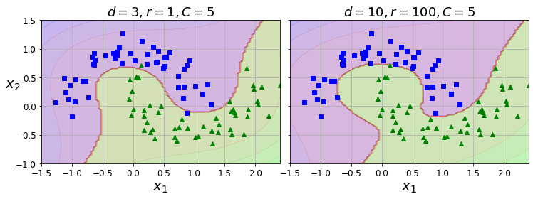
Polynomial Kernel

from sklearn.svm import SVC

poly_kernel_svm_clf = Pipeline([
        ("scaler", StandardScaler()),
        ("svm_clf", SVC(kernel="poly", degree=3, coef0=1, C=5))
    ])
poly_kernel_svm_clf.fit(X, y)

poly100_kernel_svm_clf = Pipeline([
        ("scaler", StandardScaler()),
        ("svm_clf", SVC(kernel="poly", degree=10, coef0=100, C=5))
    ])
poly100_kernel_svm_clf.fit(X, y)

fig, axes = plt.subplots(ncols=2, figsize=(10.5, 4), sharey=True)

plt.sca(axes[0])
plot_predictions(poly_kernel_svm_clf, [-1.5, 2.45, -1, 1.5])
plot_dataset(X, y, [-1.5, 2.4, -1, 1.5])
plt.title(r"$d=3, r=1, C=5$", fontsize=18)

plt.sca(axes[1])
plot_predictions(poly100_kernel_svm_clf, [-1.5, 2.45, -1, 1.5])
plot_dataset(X, y, [-1.5, 2.4, -1, 1.5])
plt.title(r"$d=10, r=100, C=5$", fontsize=18)
plt.ylabel("")

save_fig("moons_kernelized_polynomial_svc_plot")
plt.show()

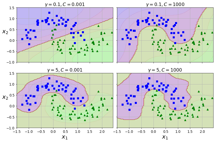
Gaussian Kernel

from sklearn.svm import SVC

gamma1, gamma2 = 0.1, 5
C1, C2 = 0.001, 1000
hyperparams = (gamma1, C1), (gamma1, C2), (gamma2, C1), (gamma2, C2)

svm_clfs = []
for gamma, C in hyperparams:
    rbf_kernel_svm_clf = Pipeline([
            ("scaler", StandardScaler()),
            ("svm_clf", SVC(kernel="rbf", gamma=gamma, C=C))
        ])
    rbf_kernel_svm_clf.fit(X, y)
    svm_clfs.append(rbf_kernel_svm_clf)

fig, axes = plt.subplots(nrows=2, ncols=2, figsize=(10.5, 7), sharex=True, sharey=True)

for i, svm_clf in enumerate(svm_clfs):
    plt.sca(axes[i // 2, i % 2])
    plot_predictions(svm_clf, [-1.5, 2.45, -1, 1.5])
    plot_dataset(X, y, [-1.5, 2.45, -1, 1.5])
    gamma, C = hyperparams[i]
    plt.title(r"$\gamma = {}, C = {}$".format(gamma, C), fontsize=16)
    if i in (0, 1):
        plt.xlabel("")
    if i in (1, 3):
        plt.ylabel("")

save_fig("moons_rbf_svc_plot")
plt.show()

---

참조: 원본코드
코드에 문제가 있거나 궁금한 점이 있으면 wjddyd66@naver.com으로 Mail을 남겨주세요.