Paper34. IntTower: the Next Generation of Two-Tower Model for Pre-Ranking System

IntTower: the Next Generation of Two-Tower Model for Pre-Ranking System

Abstract

Scoring a large number of candidates precisely in several milliseconds is vital for industrial pre-ranking systems. Existing preranking systems primarily adopt the two-tower model since the “user-item decoupling architecture” paradigm is able to balance the efficiency and effectiveness. However, the cost of high efficiency is the neglect of the potential information interaction between user and item towers, hindering the prediction accuracy critically. In this paper, we show it is possible to design a two-tower model that emphasizes both information interactions and inference efficiency. The proposed model, IntTower (short for Interaction enhanced TwoTower), consists of Light-SE, FE-Block and CIR modules. Specifically, lightweight Light-SE module is used to identify the importance of different features and obtain refined feature representations in each tower. FE-Block module performs fine-grained and early feature interactions to capture the interactive signals between user and item towers explicitly and CIR module leverages a contrastive interaction regularization to further enhance the interactions implicitly. Experimental results on three public datasets show that IntTower outperforms the SOTA pre-ranking models significantly and even achieves comparable performance in comparison with the ranking models. Moreover, we further verify the effectiveness of IntTower on a large-scale advertisement pre-ranking system. The code of IntTower is publicly available.

기존의 Pre-Ranking Model에서 많이 사용되는 Model은 Two-Tower Model이다. Two-Tower Model이란 User Embedding과 Item Embedding을 따로 구하여 Distance를 기반으로 Objective Function을 구현하는 Model이다.

하지만, 이러한 Two-Tower Model을 결국 “2-modality Model로서 치환하여 생각하게 되면 -> Late Fusion으로 인하여 Interaction Information이 손실된다는 문제점이 발생하게 된다.” (논문에서는 이러한 문제점을 “Late Interaction”이라 지칭하고 있다.)

해당 논문에서는 이러한 문제점을 해결하기 위하여 “IntTower (short for Interaction enhanced TwoTower)를 제안한다.” 해당 Model은 크게 3가지 주요한 Modulce로서 이루워져 있다.

• 1) Light-SE: 각각의 Tower (User or Item)에서 Embedding을 잘하기 위하여 사용되는 Module
• 2) FE-Block: User-Item간의 Interaction을 파악하기 위하여 사용되는 Module
• 3) CIR module: Contrastive Interaction Regularization을 통하여 Interaction을 강조하게 하는 Module

이러한 Module로 이루워진 Int-Tower Model은 Performance 뿐만 아니라 Inference속도도 빠르기 때문에, Pre-Ranking Model로서 적합하다는 것을 여러 데이터셋에서 적용하고 증명한다.

Introduction

Ranking Model에 대한 Process를 생각하면 아래의 Figure와 같다.

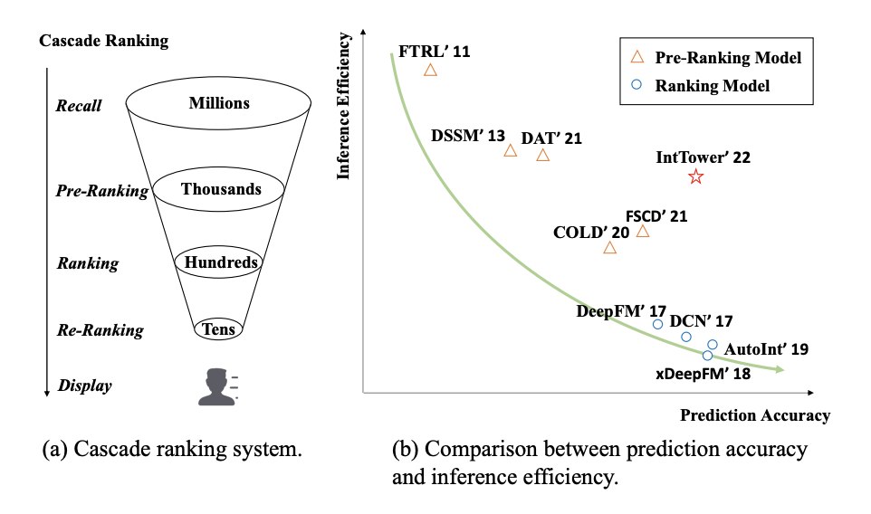
User-Item쌍이 많이 때문에 (1) Pre-Tanking (2) Ranking (3) Re-Ranking순으로 Process가 이루워 진다.
당연한 이야기로서, Model Architecture가 복잡해 질수록 Prediction Accuracy가 증가하지만, Inference Efficiency는 낮아지는 문제가 발생하게 된다. 오른쪽 Figure를 살펴보게 되면, 제안하는 IntTower Model은 Pre-Ranking Model임에도 불고하고, Ranking Model에서 대표적으로 많이 사용하는 DeepFM 보다 Accuracy는 높고 Inference 속도는 Pre-Ranking Model에서 중간 정도라는 것을 알 수 있다.

요약하면, Pre-Ranking Model의 목표는 수많은 User-Item 쌍에서 정확한 Candidate를 Generation해야 하며, 이 과정에서 (1) Inference 속도가 높아야 한다. (2) Prediction Accuracy가 높아야 한다라는 두가지 제약사항을 가지게 된다.

Preliminary

Base Model이 되는 Two-Tower Model을 Figure로 보면 아래와 같다.

위의 Figure에서 사용되는 Input과 Output을 수식으로 나타내면 아래와 같다.

• \(x = [\underbrace{x_1, x_2, \ldots, x_m}_\textrm{user-related};\underbrace{x_1, x_2, \ldots, x_n}_\textrm{item-related}]\): Input
  • \(m\): Number of user field
  • \(n\): Number of item field
• \(y \in {0, 1}\): Label(=CTR)

위의 수식에서 결국 Inner Product에서 사용하게 되는 User, Item Embedding을 구하는 식은 아래와 같다.

ex) User Embedding

1. Embedding Layer: \(e=[e_1, e_2, \ldots, e_m]\): 각각의 Field를 Look-up operation을 통하여 Embedding하는 과정이다.
   • \(e_i \in \mathbb{R}^d\)
2. FC Layer: \(h^{i+1} = \textit{relu}(W^ih^i + b^i)\): Embedding을 Deep Learning Layer를 거쳐 Embedding Diemnsion을 줄이는 과정이다.
   • \(W^i \in \mathbb{R}^{d_{i+1} \times d_i}\)
   • \(b^i \in \mathbb{R}^{d_i}\)
   • \(h^0 = e\)
   • \(d^i\): The width of the i-th FC Layer
   • \(d^0 = d \times m\)
3. Later Normalization: \(h_u = \textit{L2Norm}(h^L)\)

위와 같이 Item Embedding도 구하게 되면, 최종적인 Prediciton은 아래와 같다.

$$\hat{y} = h_u^T h_v$$

• \(h_u\): User Embedding
• \(h_v\): Item Embedding

결과적으로 문제점으로 계산되는 “Late Interaction”이란 User Embedding과 Item Embedding을 구하는 과정에서 각각의 Modality만의 정보만 사용하고, Modality간의 Interaction은 고려하지 않습니다.

IntTower

논문의 저자들이 제안하는 IntTower의 Model Architecture를 아래와 같이 제안한다.

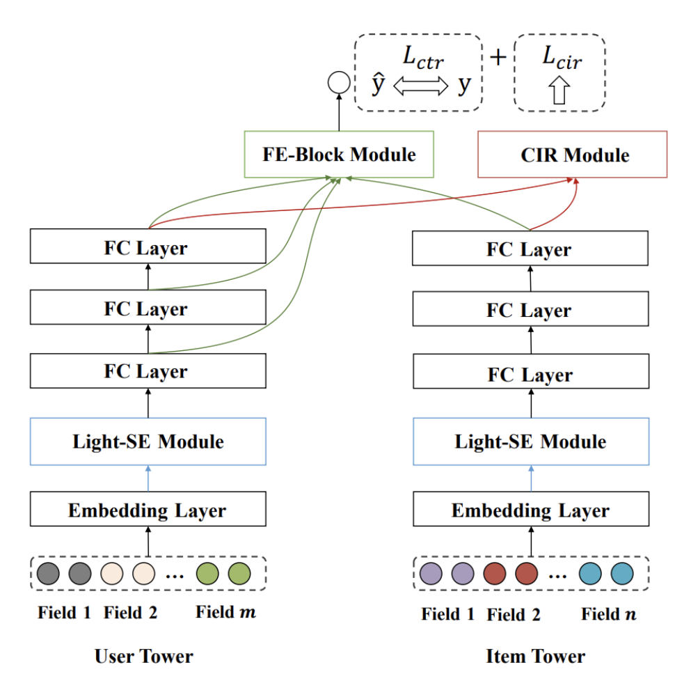
위의 Model Architecture에서 논문의 저잘들이 주요하다고 생각하는 3 가지 Module에 대하여 각각 알아보자.

Light-SE (Lightweight SENET) Block

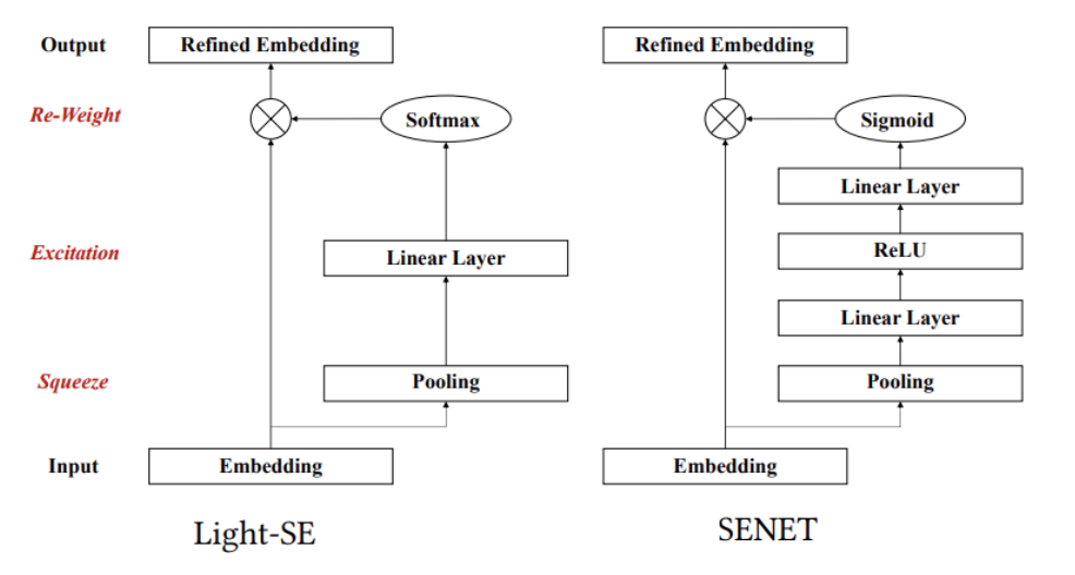
해당 Module을 이해하기 위해서는 먼저, SENET (Squeeze-and-Excitation Networks을 이해해야 한다. SENET에서 논문저자들이 조금 변형한 Module이 Light-SE이다.

먼저, SENET의 Contribution은 CNN에서 Channel간의 상호작용을 학습한 뒤, 그 정보를 사용해 채널 단위로 새로운 가중치를 줘 성능 향상을 이끌어 냈다이다. 즉, Attention을 Channel에 적용하여 Performance를 이끌어 냈다 라고 생각할 수 있다. SENET의 Architecture는 아래와 같다.

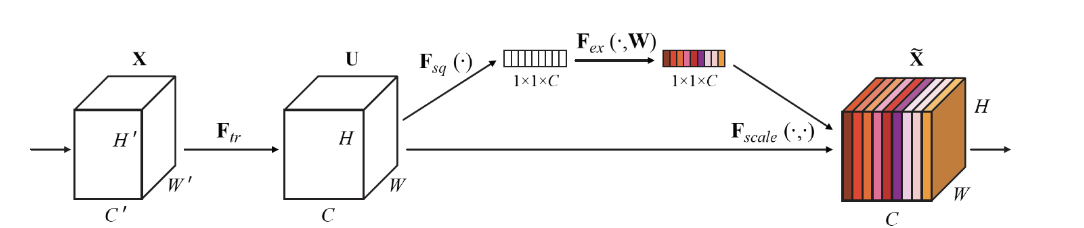
그림을 보게 되면 크게 \(F_{sq}\), \(F_{ex}\)로서 이루워 진것을 알 수 있다.

각각의 과정은 Squeeze, Excitation이라는 뜻이다. 해당 과정을 논문의 Light-SE에 적용하면 아래와 같다.

1. Squeeze:
   • Channel Dependency를 고려하기 위하여 각각의 Channel 정보를 구하는 과정.
   • 논문 Figure에서는 Pooling Layer이다.
   • Recommendation에 적용하면, 각 User/Item마다의 Field에서 대표하는 Weight값 하나로서 나타내는 과정 이다.
2. Excitation:
   • Channel Dependency를 고려하는 과정이다. 해당 과정에서의 의미는 크게 2가지 이다.
     • (1) Must be flexible: 채널간의 복잡한 non-linear 관계를 찾을 수 있어야 한다.
     • (2) Learn non-mutually-exclusive relationship: C개 채널 중 하나만 골라서 가중치를 높이는 것이 아니라, 여러 채널을 골라서 강조할 수 있어야 한다.
   • 논문 Figure에서는 Linear Layer와 Softmax를 의미하게 된다.
   • Recomendation에 적용하면, 각 User/Item마다의 Field간의 Interaction을 구할 수 있다. (아직, Single Modality의안에서 각각의 Field별로 Interaction을 구하기 위한 과정이다.)

각각의 해당 과정을 이해하기 위하여 현재, User Embedding Vector (\(e=[e_1, e_2, \ldots, e_m]\))이 있는 경우, 어떻게 Light-SE Block을 구하는지 알아보자.

Step 1. Squeeze
해당 과정은 쉽게 아래와 같이 구할 수 있다.

$$z_i = f_{sq}(e_i) = \frac{1}{d} \sum_{t=1}^d e_i^d$$

• \(z = [z_1, z_2, \ldots, z_m] \mathbb{R}^{m}\): Squeeze Embedding
  • \(z_i\): Scalar Value
• \(e_i \in \mathbb{R}^d\)

위의 수식을 살펴보게 되면, 단순히 특정 Field Embedding값을 모두 Summation한 뒤에, Dimension값으로 나눈 것 이라 할 수 있다. 이러한 의미는 각 Field를 대표할 수 있는 Scalar값 하나로 표현한 것이고 CNN에서 대입하면 Global Pooling이라고 생각할 수 있다.

Step 2. Excitation and Reweight
해당 과정은 아래와 같이 구할 수 있다.

$$k = f_{ex}(z) = \textit{softmax}(Wz + b)$$

• \(W \in \mathbb{R}^{m \times m}\)
• \(b \in \mathbb{R}^{m}\)

수식을 살펴보게 되면,

1. Linear Layer를 통하여 각 Field간의 Interaction을 구하게 되며
2. Softmax로서 각 Field의 중요도를 구하게 된다.

최종적으로 Refined된 Embedding Layer의 값은 아래와 같이 계산된다.

$$\tilde{e} = f_{rw} (k,e) = [k_1 \cdot e_1, k_2 \cdot e_2, \ldots, k_m \cdot e_m]$$

결국 Light-SE Module의 의미는 각각의 Modality (User, Item)안에서 Field간의 Interaction을 고려하였을 때, 주요한 Field의 값을 강조할 수 있다.

Appendix. Light-SE vs SENET

두 Module의 차이점을 살펴보게 되면, 2 가지 이다.

1. Number of Linear Layer
SENET에서는 Linear Layer가 2개라는 것을 알 수 있다. 해당 논문에서는 아래와 같이 구현하였다.

$$W_2 \cdot \textit{ReLU}(W_1 \cdot z)$$

• \(W_1 \in \mathbb{R}^{\frac{m}{r}, m}\)
• \(W_2 \in \mathbb{R}^{m, \frac{m}{r}}\)

해당 논문에서 이렇게 2개의 weight로서 곱하는 이유는 결과적으로 Training해야하는 Parameter를 줄이기 위하여 위와 같이 구현하였다고 하였다.

현재 적용하는 Recommendation에서는 각 File의 Embedidng Diemsion이 크지 않으면, 해당 과정이 필요없다 생각한다. 만약, Diemension이 높다면 위와 같이 변경하여 사용하여야 한다.

2. Softmax vs Sigmoid (개인적인 생각)
SENET에서 Sigmoid를 사용한 이유는 정확히 나와있지 않지만 “Learn non-mutually-exclusive relationship: C개 채널 중 하나만 골라서 가중치를 높이는 것이 아니라, 여러 채널을 골라서 강조할 수 있어야 한다.”를 만족하기 위하여 Sigmoid를 곱한 것으로 판단 된다.

하지만, 해당 논문에서는 Softmax를 사용하였다. 이는 결국 상대적인 값을 가질 수 밖에 없기 때문에 (sum=1을 만족하기 위하여) 주요한 Filed와 상대적으로 덜 중요한 Filed를 강조할 수 있는 형태로 학습되게 된다.

이러한 Module구현으로 각각의 장점과 단점이 발생한다고 생각한다.

• 장점: Single Modality관점으로 생각하였을 때, 불필요한 File의 정보를 줄일 수 있다. 즉, L2 Normalization과 같은 효과를 생각할 수 있다.
• 단점: Two Modality관점으로 생각하였을 때는 결국 Interaction에서 의미있는 Field가 이전의 Light-SE Module로 인하여 Filtering된다는 문제가 발생할 수 있다.

FE Block (Fine-grained and Early Feature Interaction Block)

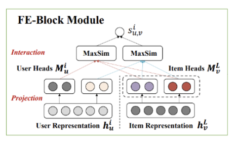
FE Block Module의 의미는 Late-Interaction의 문제를 해결하기 위하여, Early-Interaction을 함께 사용한다는 것 이다.
Model Architecture를 살펴보게 되면, 여러 User FE Later의 Output과 Item Layer FE Layer의 Output간의 관계를 고려하게 된다.
이러한 구현을 위하여 해당 논문에서는 Projection & Interaction으로서 2 step으로 구현하였다.

Projection Step
현재, 모든 수식은 아래와 같은 가정일 때의 수식 이다.

1. User Embedding을 구할때 L개의 FC Layer가 있다.
2. Item Embedding은 마지막 L FC Layer Output을 사용한다.
3. 각각의 Embedding은 H개의 Heads로서 이루워져 있다.

즉, 각각의 Embedding을 H개의 Heads로서 이루워진 Embedding으로서 바꾸어야 된다.
이러한 경우 User Embedding인 경우 L개의 Output이 모두 Dimension이 다르므로, Embedding Size를 맞추기 위하여 Projection 과정이 필요하다.

위와 같은 과정을 이해하게 되면, 아래의 수식을 쉽게 이해할 수 있다.

Projection Step 1. User Embedding

$$m_u^{i,h} = W_u^{i,h} h_u^i + b_u^{i,h}, h=1, 2, \ldots, H$$

• \(i\): 몇 번째 FC Layer의 Output인가.
• \(H\): Heads의 갯수
• \(h_u^i\): Output of i-th User FC Layer Output
• \(W_u^{i,h} \in \mathbb{R}^{d_i \times p}\): Weight
• \(b_u^{i,h} \in \mathbb{R}^{p}\): Bias
• \(m_u^{i,h} \in \mathbb{R}^{p}\): 각각의 Heads
• \(M_u^i \in \mathbb{R}^{pH} = \textit{Concat}(m_u^{i,1}, \ldots, m_u^{i,H})\)

위의 수식을 살펴보게 되면, i-th FC Layer Output의 Dimension을 맞추고, 각각의 Heads를 모아서 최종적인 Embedding을 만들게 된다.

위에서는 L개의 FC Output을 만들기 때문에 최종적인 Embedding \(M_u = [M_u^1, \ldots, M_u^L]\)으로서 생각할 수 있다.

Projection Step 2. Item Embedding

$$m_v^{L,h} = W_v^{L,h} h_u^L + b_u^{L,h}, h=1, 2, \ldots, H$$

위의 수식이 User와 다른점은 \(i\)로서 특정 FC Layer Output을 사용하는게 아니라, 마지막 Layer의 Output인 \(L\)만 사용한다.

Interaction Step
위에서 얻은 Embedding으로서 relevance score(similarity)를 구하는 방식은 아래와 같다.

$$S_{u,v}^i = \sum_{h_u=1}^H \text{max}_{h_v \in 1,2,\ldots,H} \{(m_u^{i,h_u})^T m_v^{L,h_v}\}$$

최종적인 Prediction은 아래와 같이 이루워 진다.

$$\hat{y} = \sum_{i=1}^L S_{u,v}^i$$

위의 수식을 살펴보면 아래와 같다.

1. User Heads중 특정 Head하나를 고정한다.: \(m_u^{i,h_u}\)
2. Item Heads모두와 Similairty를 구하고 가장 큰 값을 구한다.: \(\text{max}_{h_v \in 1,2,\ldots,H} \{(m_u^{i,h_u})^T m_v^{L,h_v}\}\)
3. 위의 과정을 User Heads모두에 반복하여 적용하여 Relevance Score를 구하게 된다.: \(S_{u,v}^i = \sum_{h_u=1}^H \text{max}_{h_v \in 1,2,\ldots,H} \{(m_u^{i,h_u})^T m_v^{L,h_v}\}\)
4. 3에서 얻은 과정을 User FC i-th Layer에 모두 적용한다.: \(\hat{y} = \sum_{i=1}^L S_{u,v}^i\)

Contribution: FE-Block
위의 수식을 살펴보면 아래와 같은 Contribution을 가져갈 수 있다.

1. User FC Layer의 모든 Output을 사용하므로, Late Interaction뿐만 아니라 Early Interaction까지 파악할 수 있다.
2. 기존 Bert기반의 Model들과 비슷하게, Multi-Head Attention기법을 사용하였다. 즉, User와 Item간의 Interaction이 1개인 것이 아니라 다양한 Interaction이 있다고 가정하고, 위와 같이 표현하였다.

최종적인 Loss Function은 Binary Classification인 경우 아래와 같이 이루워진다.

$$L_{ctr} = -\frac{1}{N} \sum_{i=1}^N (y_i \log(\hat{y}_i) + (1-y_i) \log (1-\hat{y}_i)))$$

CIR (Contrastive Interaction Regularization)

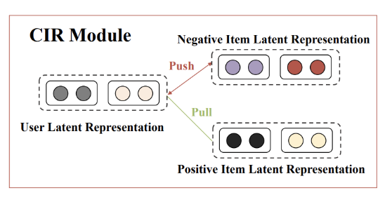
CIR Module은 “Contrastive Interaction Regularization을 통하여 Interaction을 강조하게 하는 Module” 입니다.
해당 Module의 Loss Function을 아래와 같이 InfoNCE로서 이루워져 있습니다.

$$L_{cir} = -\frac{1}{Q} \sum_{(u,v) \in Q} \text{log} \frac{\text{exp}(\text{sim}(M_u^L, M_v^L)/\tau)}{\sum_{(u', v') \in N} \text{exp}(\text{sim}(M_{u'}^L, M_{v'}^L)/\tau)}$$

• \(sim(\cdot)\): Similarity
  • \(sim(M_u^L, M_v^L) = (M_u^L)^T M_v^L / (\|M_u^L\| \cdot \| M_v^L\|)\)
• \(Q\): The total number of positive instances
• N: Total number of samples

위의 수식이 복잡해 보이지만, 하나 하나 생각해보면 쉽다.

1. CIR Loss는 User/Item FC Layer의 마지막 Output만 사용한다.: \(M_u^L, M_v^L\)
2. Negative Pair인 경우에는 값이 작을 수록 좋다. (Similarity가 낮을 수록): \(\sum_{(u', v') \in N} \text{exp}(\text{sim}(M_{u'}^L, M_{v'}^L)/\tau)\)
3. Positive Pair인 경우에는 값이 클수록 좋다.: \(\text{sim}(M_u^L, M_v^L)/\tau)\)

즉, Positive Pair인 경우에는 Similarity가 높게 학습하고, Negative Pair인 경우에는 Similarity가 작아지게 학습한다.

위의 2Loss를 활용한 최종적인 Loss Function은 아래와 같다

$$L = L_{ctr} + \lambda_1 L_{cir} + \lambda_2 \|\Theta \|_2$$

• \(\lambda_1, \lambda_2\): Hyperparameter
• \(\Theta\): Model Parameter