Paper05. Identifying diagnosis-specific genotype–phenotype associations via joint multitask sparse canonical correlation analysis and classification

\(\newcommand{\argmin}{\mathop{\mathrm{argmin}}\limits}\) \(\newcommand{\argmax}{\mathop{\mathrm{argmax}}\limits}\)

Identifying diagnosis-specific genotype–phenotype associations via joint multitask sparse canonical correlation analysis and classification

https://www.ncbi.nlm.nih.gov/pmc/articles/PMC7355274/pdf/btaa434.pdf

Abstract

Brain imaging genetics studies the complex associations between genotypic data such as single nucleotide polymorphisms (SNPs) and imaging quantitative traits (QTs).
The neurodegenerative disorders usually exhibit the diversity and heterogeneity, originating from which different diagnostic groups might carry distinct imaging QTs, SNPs and their interactions.

Problem

1. Different associaation directionality for different diagnosis groups
   • HCs and ADs could carry different imaging and genetic markers
2. The univariate methods treat each marker (SNP or QT) independently and thus they inevitably overlook the relationship within SNPs and imaging QTs
3. SCCA is unsupervised: MTSCCA => MTSSCALR
   • the diagnosis information is usually overlooked

Appendix
Quantitative trait locus (QTL) is a gene association in which multiple alleles adjacent to one locus affect gene expression, resulting in various expression traits.

Workflow

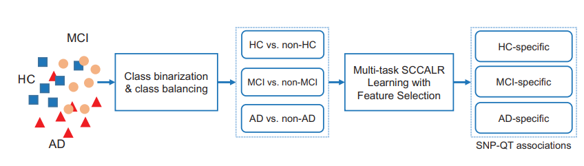
1. The whole target population is divided into different groups such as healthy control (HC), mild cognitive impairment (MCI) and AD (Problem 1)
2. The class binarization is applied to construct multiple classification tasks via the one-versus-all [OVA, or one-against-all (OAA)] decomposition strategy. (Problem 3)
3. The novel heterogeneous multitask method, i.e. the joint multitask SCCA and multitask LR, is proposed to simultaneously and systematically considering the different diagnostic groups’ relatedness. (Problem 2)
4. We obtain the dementia-related, including both MCI and AD, and the normal ageing-related imaging QTs and SNPs

Method

Dataset

• SNPs: n participants with p SNPs
• QTs: n participants with q imaging
• C: Diagnostic Groups
• genetic Data: \(X_c \in \mathbb{R}^{n*p}\)
• imaging QT Data: \(Y_c \in \mathbb{R}^{n*q}\)
• Label: \(z^l \in \mathbb{R}^{1*C}\) => Binary 0 or 1

Canocial Weight Matrix
\(U = \begin{bmatrix} u_{11} & \cdots & u_{1C} \\ \vdots & \ddots & \vdots \\ u_{p1} & \cdots & u_{pC} \end{bmatrix} \in \mathbb{R}^{p * C}\)

\(V = \begin{bmatrix} v_{11} & \cdots & v_{1C} \\ \vdots & \ddots & \vdots \\ v_{q1} & \cdots & v_{qC} \end{bmatrix} \in \mathbb{R}^{q * C}\)

Mt-SCCALR Model

$$min_{U,V} L_{LR}(V) + L_{SCCA}(U,V) + \Omega(U) + \Omega(V)$$

• \(L_{LR}(V)\): Identifies the discriminating imaging QTs byconducting multitask classification for C tasks
• \(L_{SCCA}(U,V)\): Jointly learns the bi-multivariate associations between imaging QTs and SNPs for multiple tasks.
• \(\Omega(U), \Omega(V)\): Regularization => Avoid Overfitting due to less dataset

The OVA multiclass classification via the LR

$$L_{LR}(V) = \sum_{c=1}^{C} \frac{1}{n_c} \sum_{l=1}^{n_c}[log(1+e^{y_c^l v_c})-z_{lc}y_c^l v_c]$$

• \(n_c\): The sample size for each classification task => Class balancing
• \(z_{lc}\): The corresponding class label of the lth subject for the cth task
• \(y_c^l\): The data vector of the lth subject for the cth task

Appendix: Maximum Conditional Likelihood Estimation(MLCE)

$$\hat{\theta} = \argmax_{\theta} P(D|\theta) = \argmax_{\theta} \prod_{i=1}^N P(Y_i|X_i ;\theta)$$

$$= \argmax_{\theta} log(\prod_{i=1}^N P(Y_i|X_i ;\theta)) = \argmax_{\theta} \sum_{i=1}^N log(P(Y_i|X_i ;\theta))$$

$$log(P(Y_i|X_i ;\theta)) = Y_i log(u(X_i)) + (1-Y_i)log(1-u(x)) (\because p(y|x) = u(x)^{y}(1-u(x))^{1-y})$$

$$=Y_i log(\frac{u(X_i)}{1-u(X_i)})+log(1-u(X_i))$$

$$=Y_iX_i\theta - log(1+e^{X_i\theta}) (\because X\theta = log(\frac{u(x)}{1-u(x)}))$$

$$\therefore \hat{\theta} = \argmax_{\theta}\sum_{i=1}^{N}(Y_iX_i\theta - log(1+e^{X_i\theta}))$$

The bi-multivariate association identification via the multitask SCCA

BackGround: Sparse Canonical Correlation Analysis

$$min_{w_1, ..., w_k} \sum_{i < j} -w_i^T X_i^T X_j w_j$$

$$\text{s.t. }||X_i w_i||_2^2, \Omega(w_i) \le b_i, i=1,...,I$$

Example

$$z_1 = w_{11}x_{11} + w_{12}x_{12} + ...$$

$$z_2 = w_{21}x_{21} + w_{22}x_{22} + ...$$

$$z_3 = w_{31}x_{31} + w_{32}x_{32} + ...$$

$$z_1^Tz_2 = Corr(z_1,z_2)$$

$$max_{w_1, ..., w_k} Corr(z_1,z_2) + Corr(z_1,z_3) + Corr(z_2,z_3)$$

Probelm
z1 is affected by both Term1 and Term2, so there is a high probability that it cannot be learned well.

Multitask SCCA

$$L_{SCCA}(U,V) = \sum_{c=1}^C -u_c^T X_c^T Y_c v_c$$

$$min_{u_c,v_c} \sum_{c=1}^C -u_c^T X_c^T Y_c v_c$$

$$\text{s.t. } ||X_c u_c||_2^2=1, ||Y_c v_c||_2^2=1, \forall c$$

The value of Maximum Correlation of two Vectors of the same size is the same direction.

$$min_{u_c,v_c} \sum_{c=1}^C ||u_c X_c - Y_c v_c||_2^2$$

$$\text{s.t. } ||X_c u_c||_2^2=1, ||Y_c v_c||_2^2=1, \forall c$$

Advantage

1. Calculation is performed quickly.
2. By learning about each task or modality, it overcomes the disadvantages of SCCA.

Regularization for imaging QTs via class-consistent and class-specific sparsity

Image Canocial Weight Matrix Regularization: \(\Omega(V)\)

$$\Omega(V) = \lambda_{v1}||V||_{2,1} + \lambda_{v2}||V||_{1,1} + \lambda_{v3} \sum_{c=1}^C ||v_c||_{GCL}$$

$$l_{2,1}\text{ norm}: ||V||_{2,1} = \sum_{j=1}^q ||v^j||_2 = \sum_{j=1}^q \sqrt{\sum_{c=1}^C}v_{jc}^2$$

$$l_{1,1}\text{ norm}: ||V||_{1,1} = \sum_{j=1}^q ||v^j||_1 = \sum_{j=1}^q \sum_{c=1}^C|v_{jc}|$$

The coefficieent value with a high value in all C task will converge to zero.
Only coefficient values with a high value in a specific C task will remain.

$$||v_c||_{GCL} = \sum_{j,k \in E} \sqrt{v_{jc}^2 v_{kc}^2}$$

$$E\text{: The edge set of the graph in which those highly correlated nodes are connected.}$$

Graph-Guided pairwise Group Lasso(GSL): Regualrization of the network is performed for each task. => Could capture network holding by a specific group alne

Genetic Canocial Weight Matrix Regularization: \(\Omega(U)\)

$$\Omega(U) = \lambda_{u1}||U||_{2,1} + \lambda_{u2}||U||_{1,1} + \lambda_{u3} \sum_{c=1}^C ||u_c||_{FGL}$$

$$||u_c||_{FGL} = \sum_{i=1}^{p-1}\sqrt{u_{ic}^2 + u_{(i+1)c^{'}}^2}$$

Fused pairwise group Lasso(FGL)

1. At the group level, SNPs within the same LD or gene might jointly affect the brain structure and function.

2. An important thing is that, the genetic variation might happen to patients but not HCs, resulting in that an LD structure could only exist in healthy subjects.

The optimization and convergence

$$min_{U,V} L_{LR}(V) + L_{SCCA}(U,V) + \Omega(U) + \Omega(V)$$

$$min_{U,V} \sum_{c=1}^{C} \frac{1}{n_c} \sum_{l=1}^{n_c}[log(1+e^{y_c^l v_c})-z_{lc}y_c^l v_c] + \sum_{c=1}^C ||u_c X_c - Y_c v_c||_2^2$$

$$+\lambda_{v1}||V||_{2,1} + \lambda_{v2}||V||_{1,1} + \lambda_{v3} \sum_{c=1}^C ||v_c||_{GCL}$$

$$+\lambda_{u1}||U||_{2,1} + \lambda_{u2}||U||_{1,1} + \lambda_{u3} \sum_{c=1}^C ||u_c||_{FGL}$$

$$\text{s.t. } ||X_c u_c||_2^2=1, ||Y_c v_c||_2^2=1, \forall c$$

Largrangian

$$L(U,V) = \sum_{c=1}^{C} \frac{1}{n_c} \sum_{l=1}^{n_c}[log(1+e^{y_c^l v_c})-z_{lc}y_c^l v_c] + \sum_{c=1}^C ||u_c X_c - Y_c v_c||_2^2$$

$$+\gamma_{u}(\sum_{c=1}^C ||X_c u_c||_2^2 - 1)+\gamma_{v}(\sum_{c=1}^C ||Y_c v_c||_2^2 - 1)$$

$$+\lambda_{v1}(||V||_{2,1} - \alpha_1) + \lambda_{v2}(||V||_{1,1} - \alpha_2) + \lambda_{v3} \sum_{c=1}^C (||v_c||_{GCL} - \alpha_{3c})$$

$$+\lambda_{u1}(||U||_{2,1} - \beta_1) + \lambda_{u2}(||U||_{1,1} - \beta_2) + \lambda_{v3} \sum_{c=1}^C (||u_c||_{GCL} - \beta_{3c})$$

\(\gamma_{u}, \gamma_{v}\): Tuning parameter, \(\lambda_{v1}, \lambda_{v2}, \lambda_{v3}, \lambda_{u1}, \lambda_{u2}, \lambda_{u3}\): Positive values which control model sparsity.

$$L(U,V) = \sum_{c=1}^{C} \frac{1}{n_c} \sum_{l=1}^{n_c}[log(1+e^{y_c^l v_c})-z_{lc}y_c^l v_c] + \sum_{c=1}^C ||u_c X_c - Y_c v_c||_2^2$$

$$+\gamma_{u}\sum_{c=1}^C ||X_c u_c||_2^2+\gamma_{v}\sum_{c=1}^C ||Y_c v_c||_2^2$$

$$+\lambda_{v1}||V||_{2,1} + \lambda_{v2}||V||_{1,1} + \lambda_{v3} \sum_{c=1}^C ||v_c||_{GCL}$$

$$+\lambda_{u1}||U||_{2,1} + \lambda_{u2}||U||_{1,1} + \lambda_{u3} \sum_{c=1}^C ||u_c||_{FGL}$$

U,V => Fixed => Convex & Convex in \(v_j\) convex in U,\(v_k(k \neq j)\) Fixed => Can Optimization

The solution to U

[1] Detecting genetic associations with brain imaging phenotypes in Alzheimer’s disease via a novel structured SCCA approach:https://www.sciencedirect.com/science/article/pii/S1361841520300232?via%3Dihub (Equation)
[2] Multi-Task Sparse Canonical Correlation Analysis with Application to Multi-Modal Brain Imaging Genetics: https://ieeexplore.ieee.org/stamp/stamp.jsp?tp=&arnumber=8869839 (Converge)

$$\sum_{c=1}^C ||u_c X_c - Y_c v_c||_2^2 + \gamma_{u}\sum_{c=1}^C ||X_c u_c||_2^2$$

$$+\lambda_{u1}||U||_{2,1} + \lambda_{u2}||U||_{1,1} + \lambda_{u3} \sum_{c=1}^C ||u_c||_{FGL}$$

deviation by \(u_c\)

$$-X_cY_cv_c + \lambda_{u1}\tilde{D_2}u_c + \lambda_{u2}\bar{D_2}u_c + \lambda_{u3}D_2u_c + (\gamma_u+1)X_c^TX_cu_c=0$$

• \(\tilde{D_2}=\frac{1}{2||u^i||_2}\text{ i= }(1...,p)\): Diagonal Matrix
• \(\bar{D_2}=\frac{1}{2||u_{ic}||_2}\text{ i= }(1...,p), \text{ c= }(1...,C)\): Diagonal Matrix
• \(D_2=\frac{1}{2\sqrt{u_{ic}^2+u_{(i+1)c}^2}}\text{ i= }(1...,p), \text{ c= }(1...,C)\): Diagonal Matrix

Closed Form Equation

$$u_c = (\lambda_{u1}\tilde{D_2} + \lambda_{u2}\bar{D_2} + \lambda_{u3}D_2 + (\gamma_u+1)X_c^TX_c)^{-1}X_c^TY_cv_c$$

The solution to V

$$L(U,V) = \sum_{c=1}^{C} \frac{1}{n_c} \sum_{l=1}^{n_c}[log(1+e^{y_c^l v_c})-z_{lc}y_c^l v_c] + \sum_{c=1}^C ||u_c X_c - Y_c v_c||_2^2$$

$$+\gamma_{v}\sum_{c=1}^C ||Y_c v_c||_2^2 + \lambda_{v1}||V||_{2,1} + \lambda_{v2}||V||_{1,1} + \lambda_{v3} \sum_{c=1}^C ||v_c||_{GCL}$$

$$\frac{\partial L_{LR}(V)}{\partial v_c}-2X_cY_cu_c + 2\lambda_{v1}\tilde{D_1}v_c + 2\lambda_{v2}\bar{D_1}v_c + \lambda_{v3}D_1v_c + (\gamma_v+1)X_c^TX_cu_c=0$$

Logistic Regression Term

$$\hat{\theta} = \argmax_{\theta}\sum_{i=1}^{N}(Y_iX_i\theta - log(1+e^{X_i\theta}))$$

$$\frac{\partial}{\partial \theta_j}(\sum_{i=1}^{N}(Y_iX_i\theta - log(1+e^{X_i\theta}))) =(\sum_{i=1}^{N}Y_iX_{i,j})+(-\sum_{i=1}^{N}\frac{e^{X_i\theta}X_{i,j}}{1+e^{X_i\theta}})$$

$$=\sum_{i=1}^{N}X_{i,j}(Y_i-\frac{e^{X_i\theta}}{1+e^{X_i\theta}}) =\sum_{i=1}^{N}X_{i,j}(Y_i-P(Y_i=1|X_i;\theta)) = 0$$

$$\therefore \frac{\partial L_{LR}(V)}{\partial v_c} = \frac{1}{n_c}\sum_{l=1}^{n_c}(P(z_{lc}=1|y^l_c)-z_{lc})y_{lj,c^{'}}$$

=> No close form => Second-order Deviation

$$v_c = v_c - H^{-1}(v_c)g(v_c)$$

• \(H(v_c)\): Hessian Matrix
• \(g(v_c)\): gradient(or subgradient) vector

Experiment

Hyperparameter Tuning

• \(\gamma_{u}, \gamma_{v}\): 1
• \(\lambda_{v1}, \lambda_{v2}, \lambda_{v3}, \lambda_{u1}, \lambda_{u2}, \lambda_{u3}\): Experiment => \(10^i, i: (-2, -1, 0, 1, 2) => \Upsilon \pm [0.1,0.2,...,1]\)
• Five Fold Test

Data

• ADNI1 => Focus on associations between image & SNPs, SNPs interaction
  • Image: Pet => Average, Alignment, Resample, Smoothness, Normalize => 116 ROI
  • Genotype: There were 1692 SNPs included which were collected from the neighbor of AD risk gene APOE according to the ANNOVAR annotation.
• Subject

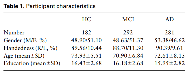
Result

Result1: Identification and interpretation of imaging QTs, SNPs

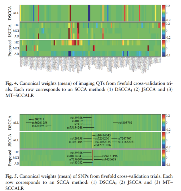
• DSCCA: Specific characteristics for Diagnosis cannot be extracted. => Because we design the model for all samples
• JSCCA: It is assumed that SCCA is used. Although we shared the features of Diagnosis, the disadvantage of SCCA is that it learns Correlation in the same direction.
• MT-SCCALR(Proposed): It can be seen that it captures specific features for Diagnosis and selects opposite features for NL and AD well.

Result2: Testomg CCCs & C;assofocation Accuracy

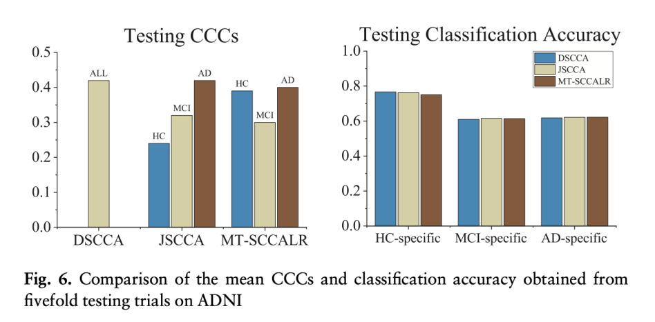
CCC(Canonical Correlation Coefficient): Measure the strength of association between two Canonical Variates:

• DSCCA: Highest CCCs as it used all sample size to yield the CCC.
• MT-SSCLR > JCCA

Accuracy: Same => The accuacy is similar, but the specific correlation for each modality and diagnosis can be designed with a high model

In the case of the current paper, the formula was completed in the form of a normal equation, which is a matrix operation, rather than a formula that enables a grid search.
This means that the feature cannot use a lot of number of samples cannot be entered.
It is also currently in bi-multimodality form.
Overcoming these two limitations seems to be the top prioirty.

Reference

[1] Multi-Task Sparse Canonical Correlation Analysis with Application to Multi-Modal Brain Imaging Genetics: https://ieeexplore.ieee.org/stamp/stamp.jsp?tp=&arnumber=8869839
[2] Identifying diagnosis-specific genotype–phenotype associations via joint multitask sparse canonical correlation analysis and classification: https://www.ncbi.nlm.nih.gov/pmc/articles/PMC7355274/pdf/btaa434.pdf