Pytorch-StyleTransfer

10 minute read

Image Style Transfer

alt text

A Neural Algorithm of Artistic Style (https://arxiv.org/abs/1508.06576)
Pretrained ResNet50
Reference below
https://discuss.pytorch.org/t/how-to-extract-features-of-an-image-from-a-trained-model/119/3
https://github.com/leongatys/PytorchNeuralStyleTransfer

위의 그림은 Image Style Transfer의 구조이다.
왼쪽의 Input으로 들어가는 것은 Style Image이다.
오른쪽의 Input으로 들어가는 것은 Content Image이다.

이번 Model에서의 핵심은 이전까지의 CNN은 최종 Feature Map을 통하여 Classifier를 통하여 Label을 선택하는 Model이였다.
하지만 Image Style Transfer는 RNN의 Embedding의 개념과 같이 Input 을 통하여 나오는 Feature Map이 Image를 대표하는 특성을 가지고 있다면 이러한 Feature를 섞어서 Image를 복원하는 작업을 하는 것 이다.

현재 논문은 각각의 3개의 Network를 통하여 Style, Content, Reconstruct를 하는 Network로 구성하고 이루워 진다.

각각의 Reconsture결과는 아래 그림과 같다.

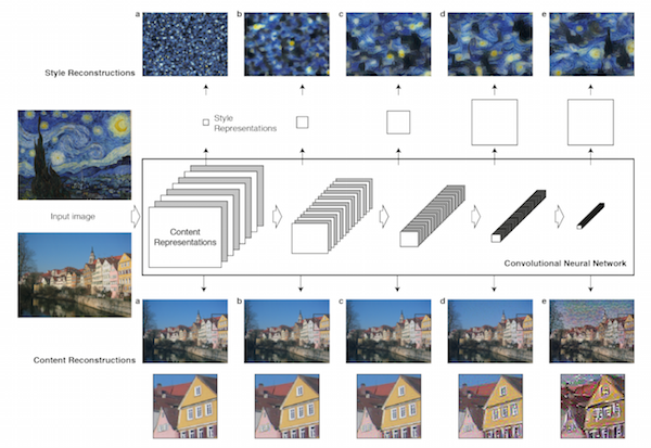
위의 그림에서 중요한 정보는 2가지 이다.

Style reconstruction에서 알 수 있는 것은 Layer가 얕을수록 원래 content정보는 거의 무시하고 ‘texture’를 복원한다.
Layer가 깊어질수록 Content의 비중이 높아진다는 것을 알 수 있다.

이러한 이유는 Style Layer는 Input Data를 Correlation을 통하여 GramMatrix로서 변환하여 대입하기 때문이다.

GramMatrix를 수식으로 표현하면 아래와 같다.

$$ G_{ij}$$

$$= \begin{bmatrix} <v_1,v_1> & <v_1,v_2> & <v_1,v_3> \\ <v_2,v_1> & <v_2,v_2> & <v_2,v_3> \\ <v_3,v_1> & <v_3,v_2> & <v_3,v_3> \\ \end{bmatrix}$$

$$= \begin{bmatrix} v_1 \\ v_2 \\ v_3 \end{bmatrix} \begin{bmatrix} v_1 & v_2 & v_3 \end{bmatrix} $$

위와 같은 과정을 Style Image에 적용시키면 다음 그림과 같다.

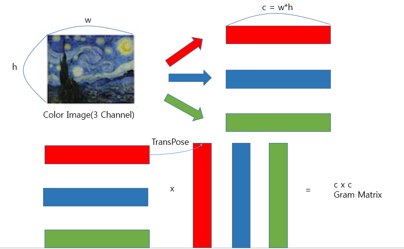
위의 그림과 같이 각각의 원소의 곱으로서 나타낼 수 있으므로 Style Layer는 Correlation의 값이라고 표현할 수 있다.

최종적인 Feature Map으로서 구성하고자하는 Image는 아래와 같은 Parameter로 정의하면 식을 쓸 수 있다.

x: Result Image
p: Content Image
a: Style Image

\[x = argmax_{x} \alpha L_{content}(p,x) + \beta L_{style}(a,x)\]

즉 Loss에 관하여 Result Image가 최대화 되는 곳을 찾으므로서 Result Image를 구성할 수 있다.

Reconstruction

Style과 Content를 각각 Reconstruction하기 위한 수식을 알아보기 전에 공통적인 Parameter를 정의하고 가자.

$S_l$: Style Input의 l번째 Layer의 Feature Map
$P_l$: Content Input의 l번째 Layer의 Feature Map
$F_l$: Result Input의 l번째 Layer의 Feature Map
$x^l$: l번째 Layer에서 복원한 Image

Content Reconstruction

$$L_{content}(p,x,l) = \frac{1}{2}\sum_{ij}(F_{ij}^{l}-P_{ij}^{l})^2$$

즉, p와x에 대해 각각 Feature map을 구하고 이 둘의 차이를 MSE로서 LossFunction을 선택한 것 이다.
이에 관하여 Content Reconsturction을 한다고 가정하면 다음과 같다.

$$x^l = argmax_{x}L_{content}(p,x,l)$$

위와 같은 식을 풀기위하여 최초의 $x^l$을 Random Image로 Initialize한다면 다음과 같다.

$$ \frac{\partial argmax_{x}L_{content}(p,x,l)}{\partial F_{ij}^l} = \begin{cases} (F_{ij}^l - P_{ij}^{l})_{ij} & \mbox{if } F_{ij}^l > 0 \\ 0 & \mbox{if } F_{ij}^l < 0 \end{cases} $$

위와 같은 식을 사용함으로써 전체 Gradient를 Back-propagation알고리즘을 사용해 간단하게 계산할 수 있다.

Style Reconstruction
Style은 Content Reconsturction과 달리 위에서 언급한 Correlation부터 계산하여야 한다.
Correlation을 계산한 Gram matrix를 식으로서 표현하면 아래와 같다.

$$G_{ij}^l = \sum_{k}F_{ik}^{l}F_{kj}^l$$

또한 Style Reconsturction의 경우 모든 Layer에서의 Feature Map을 사용한다. 즉 ‘Texture’를 표현하기 위하여 전체적인 분위기서 부터 좁은 영역의 분위기까지 모두 사용하겠다는 의미이다.
따라서 모든 Feature Map을 사용함으로 인하여 최종적인 Loss를 세우기 위한 추가적인 Parameter는 다음과 같다.

$A^l$: Style Feature Map Inner Product(Gram Vector of a) at Layer l
$G^l$: Result Feature Map Inner Product(Gram Vector of a) at Layer l
$N_l$: Feature Maps at Layer l
$M_l$: Height x width of Feature Maps at Layer l

즉 위의 Parameter를 활용하여 각 레이어 l에서의 style loss는 아래와 같이 정의된다.

$$E_l = \frac{1}{4N_l^2 M_l^2}\sum_{i,j}(G_{ij}^l-A_{ij}^l)^2$$

위의 각 Layer l에서의 Style Loss를 모두 더한 최종적인 Style Loss는 아래 식과 같다.

$$L_{style}(a,x) = \sum_{l=0}^L w_l E_l$$

각 Layer의 Loss인 $E_l$에 대하여 미분하게 된다면 다음과 같은 식을 얻을 수 있다.

$$\frac{\partial E_l}{\partial F_{ij}^l} = \begin{cases} \frac{1}{N_l^2 M_l^2}((F^l)^T(G^l - A^l))_{ji} & \mbox{if } F_{ij}^l > 0 \\ 0 & \mbox{if } F_{ij}^l < 0 \end{cases} $$

Total Loss
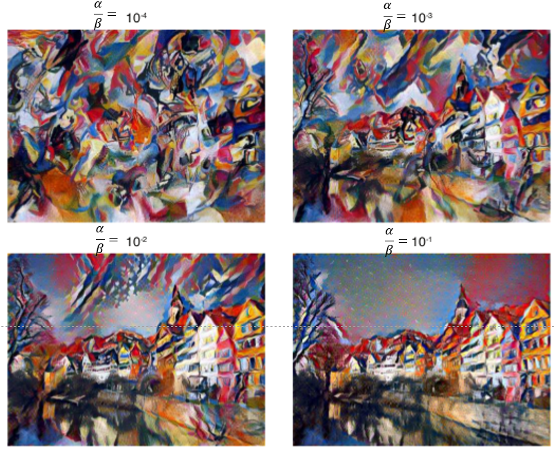
위의 Content Reconstruction에서 정리한 식과 Style Reconsturction에서 정리한 식을 통하여 전체적인 Loss를 구하게 된다면 식은 아래와 같다.

$$L_{total}(p,a,x) = \alpha L_{content}(p,x) + \beta L_{style}(a,x)$$

위의 식에서 $\alpha, \beta$ 의 가중치의 적용을 어떻게 하냐에 따라서 다음과 같은 결과물을 얻을 수 있다.

Model 구현

1. Settings

1) Import required libraries

import torch
import torch.nn as nn
import torch.optim as optim
import torch.utils as utils
import torch.utils.data as data
import torchvision.models as models
import torchvision.utils as v_utils
import torchvision.transforms as transforms
import matplotlib.pyplot as plt
from PIL import Image
%matplotlib inline

2) Hyperparameter

# 컨텐츠 손실을 어느 지점에서 맞출것인지 지정해놓습니다.
content_layer_num = 2
image_size = 512
epoch = 10000

2. Data

1) Directory

content_dir = "./image/content/1.JPG"
style_dir = "./image/style/2.jpg"

2) Prepocessing Function

전처리 함수
이미 학습된 ResNet Model은 ImageNet으로 학습된 Model이기 때문에 이에 따라 정규화가 필요하다.

즉, Input Image로 들어가는 값이 0 ~ 1사이의 값을 가지게 하기 위해서 사용하는 것 이다.
Pytorch 정식 Site에 Pre-Trained Model 사용방법에는 권고사항으로 적혀있다.

All pre-trained models expect input images normalized in the same way, i.e. mini-batches of 3-channel RGB images of shape (3 x H x W), where H and W are expected to be at least 224. The images have to be loaded in to a range of [0, 1] and then normalized using mean = [0.485, 0.456, 0.406] and std = [0.229, 0.224, 0.225]. You can use the following transform to normalize:
normalize = transforms.Normalize(mean=[0.485, 0.456, 0.406],std=[0.229, 0.224, 0.225])

Normalization 식

$$y = \frac{x-m}{\alpha}$$

# 이미 학습된 ResNet 모델이 이미지넷으로 학습된 모델이기 때문에 이에 따라 정규화해줍니다.
normalize = transforms.Normalize(mean=[0.485, 0.456, 0.406], std=[0.229, 0.224, 0.225])

def image_preprocess(img_dir):
    img = Image.open(img_dir)
    transform = transforms.Compose([
                    transforms.Resize(image_size),
                    transforms.CenterCrop(image_size),
                    transforms.ToTensor(),
                    normalize,
                ])
    img = transform(img).view((-1,3,image_size,image_size))
    return img

3) Post processing Function

후처리 함수
위에서 Input Image를 정규화 상태로 진행하였기 때문에 원본 Image를 보기 뒤해서는 뺏던 값들을 다시 더해주는 과정이 필요하다.

위에서 Normalization 식 $y = \frac{x-m}{\alpha}$을 통하여 나타내었다.
이러한 식을 다시 원상복구 시키기 위한 작업이 필요하다.

$$y = \frac{x-m}{\alpha}$$

$$\alpha y = x-m$$

$$x = \alpha(y+\frac{m}{\alpha})$$

따라서 위에서 mean = $m$, std = $\alpha$ 로 정의하였으므로 되돌리기 위해서는

$$mean = -\frac{m}{\alpha}, std = \frac{1}{\alpha}$$

이 되어야 한다.

img.clamp(0,1)

function clamp(x, min, max):
    if (x < min) then
        x = min;
    else if (x > max) then
        x = max;
    return x;
end clamp

즉 img의 값을 0 ~ 1 사이로 변화 시키는 것 이다.

torch.transpose
torch.transpose(input, dim0, dim1) → Tensor 즉 img의 dimension을 바꾸는 작업이다. 현재 Tensor로서 되어있는 값을 0 -> 1 ->2차원으로 늘려서 img를 볼 수 있게 구성하는 작업이다.

# 정규화 된 상태로 연산을 진행하고 다시 이미지화 해서 보기위해 뺐던 값들을 다시 더해줍니다.
# 또한 이미지가 0에서 1사이의 값을 가지게 해줍니다.

def image_postprocess(tensor):
    transform = transforms.Normalize(mean=[-(0.485/0.229), -(0.456/0.224), -(0.406/0.225)], std=[(1/0.229), (1/0.224), (1/0.225)])
    img = transform(tensor.clone())
    img = img.clamp(0,1)
    img = torch.transpose(img,0,1)
    img = torch.transpose(img,1,2)
    return img

3. Model & Loss Function

1) Resnet

resnet.named_children()을 통하여 ResNet Model의 직속 자식 Node들을 불러올 수 있다.

# 미리 학습된 resnet50를 사용합니다.
resnet = models.resnet50(pretrained=True)
for name,module in resnet.named_children():
    print(name)

conv1
bn1
relu
maxpool
layer1
layer2
layer3
layer4
avgpool
fc

2) Delete Fully Connected Layer

resnet.childern()으로서 자식 Node들을 불러오되 이름은 빼고 Module만 불러온다.
Module안에는 변수들이 포함되어 있다.
이때 리턴되는 값은 Generator이기 때문에 이를 리스트로 바꿔주고, 사용할 Node를 Indexing을 통하여 가져온다.
nn.Sequential()에 전달하기 위해서는 List가 아닌 List의 내용물을 전달해야 하기 때문에 * 을 붙여서 Unpacking작업을 한다.

Generator
generator 는 간단하게 설명하면 iterator 를 생성해 주는 function 이다. iterator 는 next() 메소드를 이용해 데이터에 순차적으로 접근이 가능한 object 이다. iterator 에 대한 자세한 설명은 링크에서 확인. (iterable 과 iterator 의 의미)
출처: bluese05 블로그

Unpacking
컬렉션의 요소를 여러 개의 변수에 나누어 담는 방법을 언패킹(unpacking, 풀기)이라고 부른다.

# 레이어마다 결과값을 가져올 수 있게 forward를 정의합니다.

class Resnet(nn.Module):
    def __init__(self):
        super(Resnet,self).__init__()
        self.layer0 = nn.Sequential(*list(resnet.children())[0:1])
        self.layer1 = nn.Sequential(*list(resnet.children())[1:4])
        self.layer2 = nn.Sequential(*list(resnet.children())[4:5])
        self.layer3 = nn.Sequential(*list(resnet.children())[5:6])
        self.layer4 = nn.Sequential(*list(resnet.children())[6:7])
        self.layer5 = nn.Sequential(*list(resnet.children())[7:8])

    def forward(self,x):
        out_0 = self.layer0(x)
        out_1 = self.layer1(out_0)
        out_2 = self.layer2(out_1)
        out_3 = self.layer3(out_2)
        out_4 = self.layer4(out_3)
        out_5 = self.layer5(out_4)
        return out_0, out_1, out_2, out_3, out_4, out_5

3) Gram Matrix Function

GramMatrix를 수식으로 표현하면 아래와 같다.

$$ G_{ij} = \begin{bmatrix} <v_1,v_1> & <v_1,v_2> & <v_1,v_3> \\ <v_2,v_1> & <v_2,v_2> & <v_2,v_3> \\ <v_3,v_1> & <v_3,v_2> & <v_3,v_3> \\ \end{bmatrix} = \begin{bmatrix} v_1 \\ v_2 \\ v_3 \end{bmatrix} \begin{bmatrix} v_1 & v_2 & v_3 \end{bmatrix} $$

위와 같은 과정을 Style Image에 적용시키면 다음 그림과 같다.

# 그람 행렬을 생성하는 클래스 및 함수를 정의합니다. 
# [batch,channel,height,width] -> [b,c,h*w]
# [b,c,h*w] x [b,h*w,c] = [b,c,c]

class GramMatrix(nn.Module):
    def forward(self, input):
        b,c,h,w = input.size()
        F = input.view(b, c, h*w)
        G = torch.bmm(F, F.transpose(1,2)) 
        return G

4) Model on GPU

Pre Trainned된 Resnet Parameter를 변화시키지 않기 위하여 resnet의 parameter전부를 바꾸지 않는 작업이다.
param.requires_grad = False을 통하여 Parameter가 변하는 것을 방지한다.

# 모델을 학습의 대상이 아니기 때문에 requires_grad를 False로 설정합니다.
device = torch.device("cuda:0" if torch.cuda.is_available() else "cpu")
print(device)

resnet = Resnet().to(device)
for param in resnet.parameters():
    param.requires_grad = False

cuda:0

5) Gram Matrix Loss

Style Image는 GramMatrix로 변환 후 Loss를 계산해야 하므로 따로 정의하였다.

# 그람행렬간의 손실을 계산하는 클래스 및 함수를 정의합니다.

class GramMSELoss(nn.Module):
    def forward(self, input, target):
        out = nn.MSELoss()(GramMatrix()(input), target)
        return out

4. Train

1) Prepare Images

똑같이 ResNet을 사용하나 Style과 Content는 Weight Update가 필요 없다.
그렇기 때문에 .to(device)로서 올리게 된다.
하지만 generated 즉, Style 과 Content를 합쳐서 결과물을 낼 것은 지속적인 Weight Update가 필요하기 때문에 requires_grad()를 통하여 Weight가 Update가 될 수 있게 바꾼다음 Device에 올리는 작업을 실시한다.

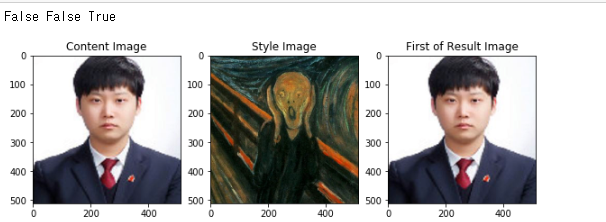
# 컨텐츠 이미지, 스타일 이미지, 학습의 대상이 되는 이미지를 정의합니다.

content = image_preprocess(content_dir).to(device)
style = image_preprocess(style_dir).to(device)
generated = content.clone().requires_grad_().to(device)

print(content.requires_grad,style.requires_grad,generated.requires_grad)

# 각각을 시각화 합니다.

plt.imshow(image_postprocess(content[0].cpu()))
plt.show()

plt.imshow(image_postprocess(style[0].cpu()))
plt.show()

gen_img = image_postprocess(generated[0].cpu()).data.numpy()
plt.imshow(gen_img)
plt.show()

2) Set Targets & Style Weights

style_target: Correlation으로서 GramMatrix를 사용하여 나타내고 모든 요소에서 뽑아내므로 Target은 for구문으로서 List로 연결
content_target: 특정 Layer의 결과값만 사용하므 resnet의 특정 Output 1개만을 사용한다.
style_weight: $L_{style}(a,x) = \sum_{l=0}^L w_l E_l$에서 $w_l$의 초기값을 설정하는 것 이다. Resnet Model에서 6개의 out_0 ~ out_6을 뽑아내므로 6개 선언

# 목표값을 설정하고 행렬의 크기에 따른 가중치도 함께 정의해놓습니다

style_target = list(GramMatrix().to(device)(i) for i in resnet(style))
content_target = resnet(content)[content_layer_num]
style_weight = [1/n**2 for n in [64,64,256,512,1024,2048]]

3) Train

style_loss: $L_{style}(a,x)$
content_loss: $L_{content}(p,x)$
total_loss: $L_{total}(p,a,x) = \alpha L_{content}(p,x) + \beta L_{style}(a,x)$

Optimizer로서는 처음보는 LBFGS를 사용하였다.
torch.optim.LBFGS(params, lr=1, max_iter=20, max_eval=None, tolerance_grad=1e-05, tolerance_change=1e-09, history_size=100, line_search_fn=None)

lr (float) – learning rate (default: 1)
max_iter (int) – maximal number of iterations per optimization step (default: 20)
max_eval (int) – maximal number of function evaluations per optimization step (default: max_iter * 1.25).
tolerance_grad (float) – termination tolerance on first order optimality (default: 1e-5).
tolerance_change (float) – termination tolerance on function value/parameter changes (default: 1e-9).
history_size (int) – update history size (default: 100).
line_search_fn (str) – either ‘strong_wolfe’ or None (default: None).

LBFGS에 기본이 되는 Newton’s Method부터 살펴보자.

Newton’s Method

Newton’s Method는 위의 그림과 같다.
결론 부터 얘기하자면
어떤 $x$에 대한 함수 $f(x)$가 존재한다고 가정하자.
$f(x) = 0$인점을 찾는 것이 목적이다.
이러한 목적을 위해서 한 점 $x_t$에서의 값을 $f(x_t)$라고 한다면
$f\prime(x_t)$와 x축과의 접점을 $x_{t+1}$이라고 하자
그렇다면 식은 아래와 같이 적용 될 수 있다.

$$f\prime(x_t) = \frac{f(x_t)-0}{x_t-x_{t+1}}$$

$$x_t - x_{t+1} = \frac{f(x_t)}{f\prime(x_t)}$$

$$x_{t+1} = x_t - \frac{f(x_t)}{f\prime(x_t)}$$

위의 식의 과정을 아래와 같은 식에 다시 적용시킨다고 하면

$$f\prime\prime(x_t) = \frac{f\prime(x_t)-0}{x_t-x_{t+1}}$$

$$x_t - x_{t+1} = \frac{f\prime(x_t)}{f\prime\prime(x_t)}$$

$$x_{t+1} = x_t - \frac{f\prime(x_t)}{f\prime\prime(x_t)}$$

즉 계속 반복하다 보면 $f\prime(x_t) = 0$인 지점 찾을 수 있다는 방식이 Newton’s Method이다.

위와 같이 2차 미분 값을 얻기 위한 $f\prime\prime(x_t)$는 시간이 $O(n^3)$이나 걸리므로 이 값을 근사하는 방식으로 바꿔서 연산 속도를 높인 방식이 바로 BFGS이다.
BFGS에서 최근 m개의 1차 미분 값만을 사용해서 더 적은 메모리를 사용하게 변형한 방법이 바로 L-BFGS이다.

L-BGFS 자세한 내용

# LBFGS 최적화 함수를 사용합니다.
# 이때 학습의 대상은 모델의 가중치가 아닌 이미지 자체입니다.

optimizer = optim.LBFGS([generated])

iteration = [0]
while iteration[0] < epoch:
    def closure():
        optimizer.zero_grad()
        out = resnet(generated)
        
        # 스타일 손실을 각각의 목표값에 따라 계산하고 이를 리스트로 저장합니다.
        style_loss = [GramMSELoss().to(device)(out[i],style_target[i])*style_weight[i] for i in range(len(style_target))]
        
        # 컨텐츠 손실은 지정한 위치에서만 계산되므로 하나의 수치로 저장됩니다.
        content_loss = nn.MSELoss().to(device)(out[content_layer_num],content_target)
        
        # 스타일:컨텐츠 = 10:1의 비중으로 총 손실을 계산합니다.
        total_loss = 10 * sum(style_loss) + torch.sum(content_loss)
        total_loss.backward()

        if iteration[0] % 100 == 0:
            print(total_loss)
        iteration[0] += 1
        return total_loss

    optimizer.step(closure)

tensor(22277024., device='cuda:0', grad_fn=<AddBackward0>)
tensor(197.4590, device='cuda:0', grad_fn=<AddBackward0>)
tensor(134.6795, device='cuda:0', grad_fn=<AddBackward0>)

...

tensor(0.5251, device='cuda:0', grad_fn=<AddBackward0>)
tensor(0.5243, device='cuda:0', grad_fn=<AddBackward0>)
tensor(0.5236, device='cuda:0', grad_fn=<AddBackward0>)

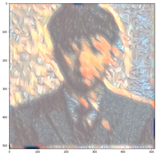
5. Check Results

# 학습된 결과 이미지를 확인합니다.

gen_img = image_postprocess(generated[0].cpu()).data.numpy()

plt.figure(figsize=(10,10))
plt.imshow(gen_img)
plt.show()

참조: 원본코드
참조: Image Style Transfer Using Convolutional Neural Networks
참조: lunit 블로그
참조: popit.kr
참조: 모두의 연구소
참조: 파이토치 첫걸음
코드에 문제가 있거나 궁금한 점이 있으면 wjddyd66@naver.com으로 Mail을 남겨주세요.

Share on

Twitter Facebook LinkedIn

JeongYong Hwang