YOLOv1(Only Concept)

YOLO v1

논문 참조: You Only Look Once: Unified, Real-Time Object Detection
Object Detection에 대한 기법은 너무 많고 Training하기 위한 시간도 많이 소요된다.
따라서 YOLO v1, v2는 Concept만 잡고 가고, YOLO v3, SSD는 직접 구현하면서 개념을 살펴보기로 한다.

(1) Introduction

YOLO또한 결과부터 살펴보면 다음과 같다.

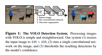
YOLO는 Image안의 Object를 Detection하여 Bounding Box로 표시하고 Classify까지 하는 기법이다.
해당 논문에서 YOLO에 대한 장점을 다음과 같이 소개하고 있다.

First, YOLO is extremely fast.
Second, YOLO reasons globally about the image when making predictions.
Third, YOLO learns generalizable representations of objects.
YOLO still lags behind state-of-the-art detection systems in accuracy.
While it can quickly identify objects in images it struggles to precisely localize some objects, especially small ones.

First, YOLO is extremely fast.
YOLO는 제목에서만 봐도 알 수 있듯이, You Only Look Once(한번만 보면 되고), Real-Time Object Detection(실시간 Object Detection)으로서 빠른것을 강조하고 있다.
YOLO가 왜 이러한 것을 부각하였는지 알아보기 위해 먼저 Object Detection에 관련된 Paper들을 시간순으로서 살펴보면 다음과 같다.

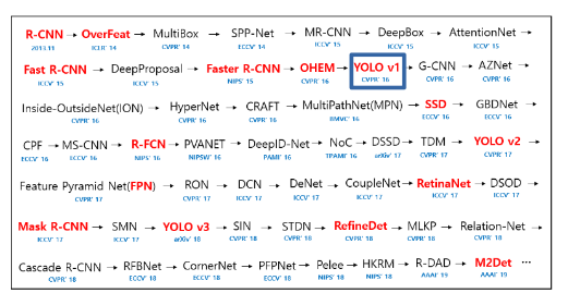
사진 출처: hoya012 GitHub

해당 Paper에서는 다음과 같이 언급하고 있다.

Current detection systems repurpose classifiers to perform detection.
To detect an object, these systems take a classifier for that object and evaluate it at various locations and scales in a test image. Systems like deformable parts models (DPM) use a sliding window approach where the classifier is run at evenly spaced locations over the entire image [10].
More recent approaches like R-CNN use region proposal methods to first generate potential bounding boxes in an image and then run a classifier on these proposed boxes.
After classification, post-processing is used to refine the bounding boxes, eliminate duplicate detections, and rescore the boxes based on other objects in the scene [13].
These complex pipelines are slow and hard to optimize because each individual component must be trained separately.

이전의 기법들은 Image Scaling을 통하여 다양한 크기의 Image에 ROI를 선정하고 ObjectDetection을 통하여 이루워지거나 Resion Proposal Network를 통하여 이루워 지기 때문에 매우 느리다고 설명한다.
그림으로서 간략하게 나타내면 다음과 같다.

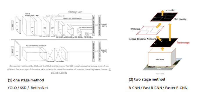
사진 출처: taeu 블로그

기존의 Object Detection기법들은 two stage method(Resion Proposal Network -> Object Detection)으로서 느리나 YOLO는 one stage method(Object Detection)으로서 속도를 매우 줄였다고 설명하고 있다.
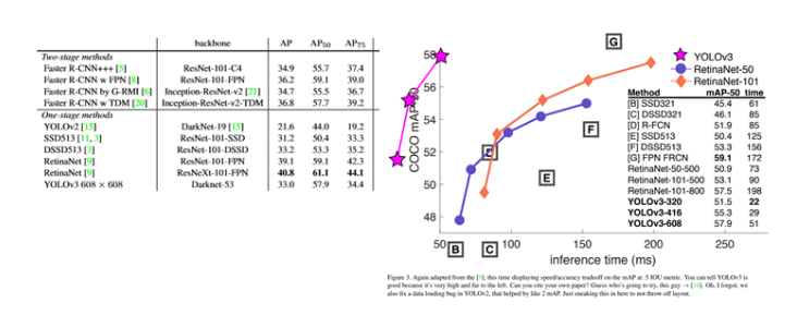
이러한 YOLO의 속도를 그래프로서 Visualization한 표는 다음과 같다.

Second, YOLO reasons globally about the image when making predictions.
YOLO기법은 Sliding Window나, Resion Proposal Network를 사용하지 않는다. 즉, Image를 잘라서 Object를 판단하지 않고 Image전체에 대하여 Encode하여 Object Detection에 사용하므로 Large Context(ex) Background)에 대하여 더 잘 판단한다고 한다.

Third, YOLO learns generalizable representations of objects.
YOLO는 매우 Generalizable한 방법이라고 소개하면서 예를 다음과 같이 들고 있습니다.

When trained on natural images and tested on artwork, YOLO outperforms top detection methods like DPM and R-CNN by a wide margin.

일반적인 사진으로서 Train을 하고 미술분야에서 Test하였을 때 다른 기법들보다 좋은 성능을 보여주었다고 합니다.
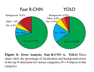
하지만, 이러한 YOLO는 몇몇 Object 특히, 작은 물체에 대하여 Localize하는 성능은 떨어진다고 얘기하고 있습니다.

(2) Unified Detection

먼저 YOLO의 작동방식을 살펴보면 다음과 같다.

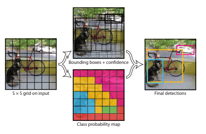
위의 사진은 다음과 같은 과정으로서 진행된다.

1) Input Image를 SxS개의 사각형(grid)로서 불리한다 이러한 사각형은 grid cell이라 불리며, 물체를 찾고, 인식(분류)하는 역할을 가지고 있다.

2) grid cell을 통하여 B개의 bounding box를 생성한다.
B개의 Bounding box를 생성하는 과정을 그림으로 표현하면 다음과 같다.

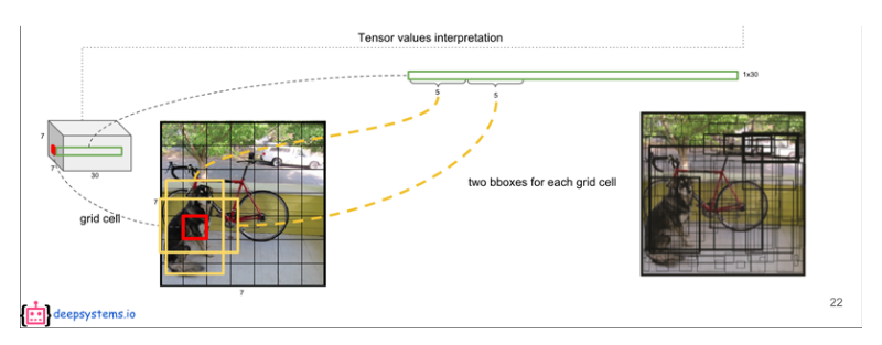
사진 출처: curaai00 블로그
즉, Grid Cell로서 Object의 Bounding Box가 될 수 있는 후보를 찾아내는 단게라고 할 수 있다.

3) Bounding Box(B)안의 Object를 예측한다.
먼저 Bounding Box는 (x,y,w,h,confidence)로서 이루워져 있다.

• x,y: Bounding Box의 중심좌표
• w,h: Bounding Box의 높이와 너비(Image의 Size에 따라서 Normalization -> x,y또한 0~1로서 Normalization)
• confidence: 해당 Bounding Box가 어떤 Object를 가지고 있고, 그 예측 %를 표시한다.

Confidence Score에 대해서 자세히 알아보면 다음과 같다.

$$Pr(Class_i|Object)*Pr(Object)*IOU^{truth}_{pred} = Pr(Object)*IOU^{truth}_{pred}$$

위의 식에서 왼쪽의 식의 의미를 살펴보면 다음과 같다.

• \(Pr(Object)\): Bounding Box가 Object를 가지고 있을 확률(Object가 없으면 0)
• \(IOU^{truth}_{pred}\)(Intersection Over Union): 예측한 box와 실제 Object가 있는 box가 얼마나 같은지
• \(Pr(Class_i|Object)\): Classify Model에서 해당 Object를 어떤 Class로 분류하고 정확도는 얼마인지

위에서 주의하여할 점은 Pr()은 Bounding Box가 아니라 Bounding Box를 구성하는 각각의 Grid Cell에 대한 Probability의 값 이다.

이러한 YOLO기법을 PASCAL VOC로 평가((2) Unified Detection의 그림 예시)하게 되면 다음과 같은 Tensor로서 Prediction이 된다.

$$S*S*(B*5+C) = 7*7*(2*5+20) = 7*7*30$$

• S: Input Image를 나누는 기준
• B: Bounding Box 개수
• C: Label Class개수

(2-1) Network Design

YOLO Model의 Network Architecture를 살펴보면 다음과 같다.

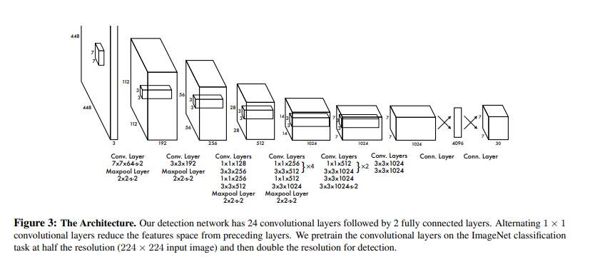
GoogleNet의 영감을 받아서 Architecture를 구성하였다고 한다.
총 24개의 Convolution Layer와 2개의 Fully Connected Layer(Fast YOLO는 Compact한 9개의 Layer로서 구성)로서 구성되어있고 Inception Module을 전부 사용하는 것이 아닌 3x3 conv뒤에 따라오는 1x1 reduction conv Layer를 추가하였다고 한다.(1x1 Convolution Layer를 사용하는 이유는 위의 Inception Link를 참조하자.)
최종적인 Model의 결과로서 448x448 Input Image -> Model -> 7x7x30 tensor of prediction으로서 구성된다.

(2-2) Training

Training을 하기전에 다음과 같은 사전작업이 필요하다.

1. 24개의 Convolution Layer에서 4개를 제거한 20개의 ConvolutionLayer + Pooling Layer + Fully Connected Layer로서 1000개의 Class를 구별하는 Model을 Training시킨다.
2. Network의 Input을 224x224에서 448x448로서 향상시킨다. Object Detection을 위한 해상도를 높이기 위한 작업이다. (개인적으로는 YOLO의 단점이라는 Small Object를 Detection을 더 잘하게 하기 위해서 작은 Image로서 상세하게 Training하고 Image의 Size가 큰 것을 Input으로 넣어서 더 쉽게 Object를 Detection하게 하기 위해서 인 것 같다.)
3. (2-1) Network Design의 Model Architecture로서 변형한다. 즉, Pooling Layer + Fully Connected Layer제거 -> 4 Convolution Layer추가 + 2개의 Fully Conntected Layer 추가. 추가한 Layer의 Weight는 Random하게 초기화 시킨다.
4. 마지막 Layer는 Bounding Box는 (x,y,w,h,confidence)에서 x,y,confidence를 예측한다.(w,h는 위에서 448,448로서 구하였다.)
5. x,y는 w,h를 통하여 0~1사이의 값을 가지도록 변경한다.
6. 마지막 Layer는 Linear한 Activation Function을 사용하고 다른 Activation Function은 조정된 Leaky ReLU를 사용한다.

$$ \phi(\theta)= \begin{cases} x, & \mbox{if }x>0 \\ 0.1x, & \mbox{otherwise} \end{cases} $$

위의 과정을 통하여 Network Architecture에 대한 작업은 끝났다.
이제 Loss Function을 알아보기 앞서 먼저 최종적인 Loss Function의 식을 살펴보자.

$$\lambda_{coord} \sum_{i=0}^{S^2} \sum_{j=0}^{B} \mathbb{1}_{ij}^{obj}[(x_i-\hat{x_i})^2 + (y_i - \hat{y_i})^2]$$

$$+\lambda_{coord} \sum_{i=0}^{S^2} \sum_{j=0}^{B} \mathbb{1}_{ij}^{obj}[(\sqrt{w_i}-\sqrt{\hat{w_i}})^2 + (\sqrt{h_i} - \sqrt{\hat{h_i}})^2]$$

$$+\sum_{i=0}^{S^2} \sum_{j=0}^{B} \mathbb{1}_{ij}^{obj}(C_i-\hat{C_i})^2$$

$$+\lambda_{noobj} \sum_{i=0}^{S^2} \sum_{j=0}^{B} \mathbb{1}_{ij}^{noobj}(C_i-\hat{C_i})^2$$

$$+\sum_{i=0}^{S^2}\mathbb{1}_{i}^{obj} \sum_{c \in classes} (p_i(c)-\hat{p_i}(c))^2$$

= Location of Bounding Box Loss + Size of Bounding Box Loss + Object Loss + Classification Loss

위의 식을 좀 더 알아보기 쉽게 시각화 하면 다음과 같다.

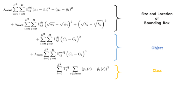
사진 출처: taeu 블로그

위의 4개의 Loss에서 공통적으로 사용하는 Parameter에 대해서 정리하면 다음과 같다.

• S: Image의 가로 세로 Grid Cell로 나눌 갯수, \(S^2\)은 모든 Grid Cell을 의미한다.
• B: Number of Bounding Box
• \(\mathbb{1}_{i}^{obj}\): Object가 존재하는 grid cell i
• \(\mathbb{1}_{ij}^{obj}\): Object가 존재하는 grid cell i의 bounding box predictor j
• \(\mathbb{1}_{ij}^{noobj}\): Object가 존재하지 않는 grid cell i의 bounding box predictor j
• \(\lambda_{coord}\)(논문에서는 5로서 정의): Object Loss와 Class Loss와 크기를 같기 하기 위하여 Location에 대한 Loss는 5를 곱하여 향상시킨다.
• \(\lambda_{noobj}\)(논문에서는 0.5로서 정의): 대부분의 Image에서 가장 많이 차지하는 것은 Background일 것이다. 즉, Object를 포함하지 않고 있는 것 이다. 이러한 Grid Cell에 대한 Confidence는 0점이 될 것이고(\(\because Pr(Class_i|Object)*Pr(Object)*IOU^{truth}_{pred} \text{ 에서 }Pr(Object)=0\)), 따라서 많은 Gradient를 사용하지 못하여 학습 초기에 분산하게 될 확률이 높다. 따라서 Object가 존재하는 것과 존재하지 않는 것에 대하여 각각의 가중치를 달리 해야 한다.

또한 Optimize하기 쉽게 sum-squared error(MSE)를 사용하였다. 이제 위의 식을 하나하나 풀면 다음과 같다.

Location of Bounding Box Loss

$$\lambda_{coord} \sum_{i=0}^{S^2} \sum_{j=0}^{B} \mathbb{1}_{ij}^{obj}[(x_i-\hat{x_i})^2 + (y_i - \hat{y_i})^2]$$

단순하게 Prediction Bounding Box의 중심과 Label의 Bounding Box의 중심을 MSE로서 계산한다.

Size of Bounding Box Loss

$$\lambda_{coord} \sum_{i=0}^{S^2} \sum_{j=0}^{B} \mathbb{1}_{ij}^{obj}[(\sqrt{w_i}-\sqrt{\hat{w_i}})^2 + (\sqrt{h_i} - \sqrt{\hat{h_i}})^2]$$

큰 Box에서의 작은 편차가 작은 Box에서의 작은편차보다 덜 중요하다. 즉, Object를 찾는 Box의 크기가 작으면 작을수록 좋기 때문에 큰 Box와 작은 Box의 편차의 차이를 줄이기 위하여 w,h의 제곱근을 사용하여 계산한다.
실제 계산을 위해 다음과 같은 Python Code를 작성하고 실행하면 제곱근을 사용하게 되면 작은 Box의 작은 편차가 더 커지는 것을 확인할 수 있다.

a_1 =[0.9,0.9]
b_1 = [1,1]

a_2 = [0.4,0.4]
b_2 = [0.5,0.5]

result1 = (a_1[0]-b_1[0])**2 + (a_1[1]-b_1[1])**2
result2 = (a_2[0]-b_2[0])**2 + (a_2[1]-b_2[1])**2
print('%.3f' %result1) #0.020
print('%.3f' %result2) #0.020
print('%.3f' %(result1-result2)) #0.000
print()

result1 = (a_1[0]**(0.5)-b_1[0]**(0.5))**2 + (a_1[1]**(0.5)-b_1[1]**(0.5))**2
result2 = (a_2[0]**(0.5)-b_2[0]**(0.5))**2 + (a_2[1]**(0.5)-b_2[1]**(0.5))**2
print('%.3f' %result1) #0.005
print('%.3f' %result2) #0.011
print('%.3f' %(result1-result2)) #-0.006

위의 두 식을 합하면(Location of Bounding Box Loss + Size of Bounding Box Loss) 위에서 정의하였던 \(IOU^{truth}_{pred}\)(예측한 box와 실제 Object가 있는 box가 얼마나 같은지)에 관한 Loss가 되는 것을 확인할 수 있다.

Object Loss

$$\sum_{i=0}^{S^2} \sum_{j=0}^{B} \mathbb{1}_{ij}^{obj}(C_i-\hat{C_i})^2 + \lambda_{noobj} \sum_{i=0}^{S^2} \sum_{j=0}^{B} \mathbb{1}_{ij}^{noobj}(C_i-\hat{C_i})^2$$

각각의 Grid Cell에서 Object가 존재할 확률(\(Pr(Object)\))을 구한다.
Label의 Data(\(C_i\))는 다음과 같다.

$$ C_i= \begin{cases} 1, & \mbox{Object가 존재하는 경우, }\mathbb{1}_{ij}^{obj} \\ 0, & \mbox{Object가 존재하지 않는 경우, }\mathbb{1}_{ij}^{noobj} \end{cases} $$

Classification Loss

$$\sum_{i=0}^{S^2}\mathbb{1}_{i}^{obj} \sum_{c \in classes} (p_i(c)-\hat{p_i}(c))^2$$

Object가 존재하는 Grid Cell i에 대하여 실제 Class일 확률을 구한다.

$$ p_i(c)= \begin{cases} 1, & \mbox{Correct Class} \\ 0, & \mbox{otherwise} \end{cases} $$

위와 같은 Loss Function에 대하여 해당 논문은 다음과 같이 설명하고 있습니다.

Note that the loss function only penalizes classification error if an object is present in that grid cell (hence the conditional class probability discussed earlier).
It also only penalizes bounding box coordinate error if that predictor is “responsible” for the ground truth box (i.e. has the highest IOU of any predictor in that grid cell).

1. Classification error는 Object가 존재하는 Grid Cell(\(\mathbb{1}_{i}^{obj}\))에 의해 영향을 받는다.
2. Bounding box coordinate error(Location of Bounding Box Loss, Size of Bounding Box Loss)는 오직 Ground truth box(Label Bounding Box, \((x_i,y_i,w_i,h_i)\))에 의해서만 영향을 받는다.

추가적인 Network의 구성은 다음과 같다.

• Momentum: 0.9 and a decay of 0.0005
• Learning Rate: [0.001, 0.01, 0.001, 0.0001] ( 처음에 0.001에서 서서히 감소시키다 75 - epoch동안 0.01, 30 epoch동안 0.001, 마지막 30 epoch동안 0.0001)
• Dropout Rate: 0.5
• Data augmentation: random scailing and translations of up to 20% of the original image size
  

(2-3) Limitation of YOLO

1. Grid Cell마다의 One Class를 예측하는 방법이기 때문에 Object주변에 작은 Object가 많이 포함되는 경우 작은 Object를 Detection하기 어렵다.
2. General한 Model이기 때문에 Unusual aspect rations or configuration와 같이 새로운 Object에 대한 Detection을 하기 어렵다.
3. Localization에 대한 부정확한 경우, 즉, 위에서 LossFunction을 정의할 때 Bounding box coordinate error(Location of Bounding Box Loss, Size of Bounding Box Loss)에 대하여 “큰 Box에서의 작은 편차가 작은 Box에서의 작은편차보다 덜 중요하다. 즉, Object를 찾는 Box의 크기가 작으면 작을수록 좋기 때문에 큰 Box와 작은 Box의 편차의 차이를 줄이기 위하여 w,h의 제곱근을 사용하여 계산한다”라고 설명하였다. 즉, 큰 Box에서의 작은 Error는 영향을 잘 안미치지만 작은 Box이면 작은 Error또한 \(IOU^{truth}_{pred}\)에 대하여 크게 영향을 미친다.

---

참조: You Only Look Once: Unified, Real-Time Object Detection
참조: taeu 블로그

코드에 문제가 있거나 궁금한 점이 있으면 wjddyd66@naver.com으로 Mail을 남겨주세요.