
Classify Structured data with feature columns
Classify Structured data with feature columns
Tensorflow 2.0에 맞게 다시 Tensorflow를 살펴볼 필요가 있다고 느껴져서 Tensorflow 정식 홈페이지에 나와있는 예제부터 전반적인 Tensorflow 사용법을 먼저 익히는 Post가 된다.
필요한 Library Import
1
2
3
4
5
6
7
8
9
10
11
12
from __future__ import absolute_import, division, print_function, unicode_literals

import io
import requests
import numpy as np
import pandas as pd

import tensorflow as tf

from tensorflow import feature_column
from tensorflow.keras import layers
from sklearn.model_selection import train_test_split
Data Preprocessing
ML과 Deep Learning을 하면서 공통적으로 제일 중요하다고 생각하는 부분은 Data Preprocessing이다.
어떻게 Data를 전처리 하냐에 따라서 같은 Model을 사용하더라도 성능차이는 많이 나게 된다.
따라서 Tensorflow 2.0 Tutorial에서도 이러한 Data를 3가지의 대표적인 유형으로 나누어서 소개하게 된다.
이번 Post Classify Structured data with feature columns는 구조화된 제일 기본적인 Data를 Keras를 사용하여 전처리 하는 Post가 된다.
이러한 Post는 4가지의 목표를 가지고 있다.
- Pandas를 사용하여 CSV 파일을 읽기
- tf.data를 사용하여 행을 섞고 배치로 나누는 입력 파이프라인을 만들기
- Load and preprocess Data
- Load and preprocess Data2
- CSV의 열을 feature_columns을 사용해 모델 훈련에 필요한 특성으로 매핑하기
- 케라스를 사용하여 모델 구축, 훈련, 평가하기
참고
이번 Post는 위의 링크인 Load and preprocess Data1, 2와 많은 부분이 겹치게 됩니다.
복습하는 차원에서 다시 한번 정리하는 Post이므로 위의 링크를 보시고 이해가 되신 분들은 이번 Post는 넘기셔도 됩니다.
The Dataset
Cleveland Clinic Foundation for Heart Disease의 Dataset을 사용하게 됩니다.
각각의 Dataset은 다음과 같은 특성을 가지게 됩니다.
중요한점은 수치형과 범주형 열이 모두 존재한다는 것 이다.
- 범주형(Categorical Data): 몇 개의 범주로 나누어 진 자료 ex) 남/여, 성공/실패
- 명목형 자료: 순서와 상관 없는 자료(단순한 분류)
- 순서형 자료: 순서와 상관 있는 자료
- 수치형(Numerical Data)
- 이산형 자료: 이산적인 값을 갖는 데이터
- 연속형 자료: 연속적인 값을 갖는 데이터
| Column | Description | Feature Type | Data Type |
|---|---|---|---|
| Age | Age in years | Numerical | integer |
| Sex | (1 = male; 0 = female) | Categorical | integer |
| CP | Chest pain type (0, 1, 2, 3, 4) | Categorical | integer |
| Trestbpd | Resting blood pressure (in mm Hg on admission to the hospital) | Numerical | integer |
| Chol | Serum cholestoral in mg/dl | Numerical | integer |
| FBS | (fasting blood sugar > 120 mg/dl) (1 = true; 0 = false) | Categorical | integer |
| RestECG | Resting electrocardiographic results (0, 1, 2) | Categorical | integer |
| Thalach | Maximum heart rate achieved | Numerical | integer |
| Exang | Exercise induced angina (1 = yes; 0 = no) | Categorical | integer |
| Oldpeak | ST depression induced by exercise relative to rest | Numerical | float |
| Slope | The slope of the peak exercise ST segment | Numerical | integer |
| CA | Number of major vessels (0-3) colored by flourosopy | Numerical | integer |
| Thal | 3 = normal; 6 = fixed defect; 7 = reversable defect | Categorical | string |
| Target | Diagnosis of heart disease (1 = true; 0 = false) | Classification | integer |
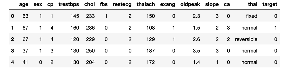
Use Pandas to create a dataframe
Pandas를 활용하여 위의 Dataset을 Dataframe형태로 변현한다.
참고(Request Error)
현재 Tensorflow 2.0에서 제공하는 Code를 그대로 사용하는 경우 Request Error가 발생하게 된다.
Pandas Version Error인지 Jupyter Notebook의 Ipython Error인지는 파악되지 않으나 Stack Overflow를 참조하여 Code를 아래와 같이 변경하여 해결하였다.
1
2
3
4
5
6
URL = 'https://storage.googleapis.com/applied-dl/heart.csv'
# Download and read Dataset
x = requests.get(url=URL).content
dataframe = pd.read_csv(io.StringIO(x.decode('utf8')))
# Top 5 Data Check
dataframe.head()
Split the dataframe into train, validation, and test
위에서 선언한 Dataframe을 활용하여 Model에 필요한 Train, Validation, and Test Dataset으로서 sklearn을 활용하여 Split을 하게 된다.
1
2
3
4
5
6
7
8
# Split the dataframe into train, validation, and test
train, test = train_test_split(dataframe,test_size=0.2)
train, val = train_test_split(train,test_size=0.2)

# Check the Split Data
print(len(train),'train examples')
print(len(val),'validation examples')
print(len(test),'test examples')
193 train examples
49 validation examples
61 test examples
Create an input pipeline using tf.data
tf.data를 활용하여 Feature, Label로서 나누고 Batch처리 까지 진행하게 된다. Model의 성능을 향상시키기 위하여 Train Dataset의 경우에는 Shuffle까지 진행하게 된다.
아래 Code가 이해되지 않으면 밑의 두 링크를 참조하도록 하자.
1
2
3
4
5
6
7
8
9
10
11
12
13
14
15
16
17
18
19
20
21
22
23
24
25
def df_to_dataset(dataframe, shuffle=True, batch_size=32):
    dataframe = dataframe.copy()
    # Pop Label
    labels = dataframe.pop('target')
    # Datafrmae to Tensor
    ds = tf.data.Dataset.from_tensor_slices((dict(dataframe),labels))
    # Shuffle Tensor
    if shuffle:
        ds = ds.shuffle(buffer_size = len(dataframe))
    # Batch Tensor
    ds = ds.batch(batch_size)
    return ds

batch_size = 5
# Train Data with Shuffle
train_ds = df_to_dataset(train,batch_size=batch_size)
# Validation Data, Test Data with no shuffle
val_ds = df_to_dataset(val,shuffle=False,batch_size=batch_size)
test_ds = df_to_dataset(test,shuffle=False,batch_size=batch_size)

# Check Tensor
for feature_batch, label_batch in train_ds.take(1):
    print('Every Feature: ',list(feature_batch.keys()))
    print('A batch of ages: ', feature_batch['age'])
    print('A batch of targets: ',label_batch)
Every Feature:  ['age', 'sex', 'cp', 'trestbps', 'chol', 'fbs', 'restecg', 'thalach', 'exang', 'oldpeak', 'slope', 'ca', 'thal']
A batch of ages:  tf.Tensor([61 64 57 41 63], shape=(5,), dtype=int32)
A batch of targets:  tf.Tensor([0 1 0 0 1], shape=(5,), dtype=int32)
Demonstrate several types of feature column
train_ds를 계속하여 Input으로 넣으나, tf.keras.layers.DenseFeatures를 사용하여 Feature Columns가 어떻게 변형되는지 살펴본다.
즉, 원하는 Dataframe의 Column을 Input으로 넣어서 어떻게 DenseFeaures로 표현되는지 살펴본다.
1
2
3
4
5
6
7
# Use this batch to demonstrate several types of feature columns
example_batch = next(iter(train_ds))[0] # Not use Label

# Create a Feature column and transform a batch of data
def demo(feature_column):
    feature_layer = layers.DenseFeatures(feature_column)
    print(feature_layer(example_batch).numpy())
Numeric columns
가장 간단한 Numeric columns이다. 기본적인 Input Data를 그대로 표현하여 나타내는 것 이다.
참조: tf.feature_column.numeric_column 사용법
참조: Option을 사용하여 Data의 수치를 바로 변경하는 것이 가능하다.(즉, 평균과 분산을 알게 되면 Normalization을 바로 적용시킬 수 있다.)
1
2
3
4
5
6
7
8
9
10
11
12
13
14
# Ignore Warning Change Backend to float 64
tf.keras.backend.set_floatx('float64')

# Check Numeric Column
age = feature_column.numeric_column('age')
print('Check NUmeric Column')
demo(age)
print()

# Check Option
normalizer_function = lambda x:(x-3)
age = feature_column.numeric_column('age',normalizer_fn=normalizer_function)
print('Check Option')
demo(age)
Check NUmeric Column
[[66.]
 [63.]
 [51.]
 [40.]
 [46.]]

Check Option
[[63.]
 [60.]
 [48.]
 [37.]
 [43.]]
Bucketized columns
위와 같은 Numeric한 수치를 바로 넣는 것이 아니라 일정한 버킷(Bucket)으로 나눌 수 있다.
즉, 일정한 번위안의 속하면 1, 아니면 0 으로서 One-Hot-Encoding형식으로서 나타내어 Bucketized Columns로 나타낼 수 있다.
참조: tf.feature_column.bucketized_column 사용법
1
2
age_buckets = feature_column.bucketized_column(age,boundaries=[18,25,30,40,45,50,55,60,65])
demo(age_buckets)
[[0. 0. 0. 0. 0. 0. 0. 0. 1. 0.]
 [0. 0. 0. 0. 0. 0. 0. 0. 1. 0.]
 [0. 0. 0. 0. 0. 1. 0. 0. 0. 0.]
 [0. 0. 0. 1. 0. 0. 0. 0. 0. 0.]
 [0. 0. 0. 0. 1. 0. 0. 0. 0. 0.]]
Categorical columns
범주형 데이터(Cateforical Data)의 경우 Model의 Input으로 넣기 위하여 수치형 데이터(Numerical Data)로 변경하여야 한다.
위의 Bucketized columns와 마찬가지로서 Category에 따라서 One-Hot-Encoidng으로서 나타낸다.
참조: tf.feature_column.indicator_column: 기본적으로 Categorical Column을 Input으로 넣기 위해서는 .indicator_column가 필요하다.
참조: tf.feature_column.catrgorical_column_with_vocabulary_list 사용법(List로서 전달)
참조: tf.feature_column.catrgorical_column_with_vocabulary_file 사용법(File로서 전달)
1
2
3
4
5
6
7
8
9
10
# Check Categorical Value
thal_category = set(dataframe['thal'])
print('Thal Catrgory')
print(thal_category)
print()

# Categorical Columns -> Numeric Tensor
thal = feature_column.categorical_column_with_vocabulary_list('thal',['fixed','normal','reversible','1','2'])
thal_one_hot = feature_column.indicator_column(thal)
demo(thal_one_hot)
Thal Catrgory
{'1', 'normal', 'reversible', 'fixed', '2'}

[[0. 1. 0. 0. 0.]
 [0. 1. 0. 0. 0.]
 [0. 1. 0. 0. 0.]
 [0. 0. 1. 0. 0.]
 [0. 1. 0. 0. 0.]]
Embedding columns
Category의 수가 매우 많아지게 되었을 경우 One-Hot-Encoding으로서 나타내는 것은 Resource를 많이 낭비하게 되고, Computing Power가 버티지 못할 확률이 매우 높아진다.
따라서 Embedding Columns로서 나타내는 것이 필요하다.
개인적인 경험으로는 이러한 Embedding Layer는 자연어 분야에서 Vocab File의 전처리를 위하여 많이 사용되는 것으로 알 고 있다.
참조: Embedding 자세한 내용
참조: tf.feature_column.embedding_column 사용법
1
2
thal_embedding = feature_column.embedding_column(thal,dimension=3)
demo(thal_embedding)
[[-0.04294701  0.6549929   0.1659287 ]
 [-0.04294701  0.6549929   0.1659287 ]
 [-0.04294701  0.6549929   0.1659287 ]
 [ 0.6932911   0.52152395 -0.26704228]
 [-0.04294701  0.6549929   0.1659287 ]]
Hashed feature columns
위와 같이 많은 Category의 수를 줄이기 위한 방법으로서 Hash Feature Columns를 사용하는 방법이 있다.
하지만, 어떻게 Hash를 할당하는 지는 자세히 모르겠으며, 다른 문자열이 같은 Bucket에 할당 될 수 있는 매우 큰 단점이 존재하나, 일부 데이터셋 에서 잘 작동한다고 한다.
참조: tf.feature_column.categorical_column_with_hash_bucket 사용법
1
2
3
thal_hashed = feature_column.categorical_column_with_hash_bucket(
      'thal', hash_bucket_size=2)
demo(feature_column.indicator_column(thal_hashed))
[[0. 1.]
 [0. 1.]
 [0. 1.]
 [1. 0.]
Crossed Feature columns
여러 특성을 연결하여 하나의 특성으로 만드는 것을 feature cross라고 한다.
모델이 특성의 조합에 대한 가중치를 학습할 수 있다.
1
2
3
4
5
6
7
8
9
10
11
12
13
# Check Thal's Categorical Value
thal_category = set(dataframe['thal'])
print('Thal Catrgory')
print(thal_category)
print()

# Check Age bucket
print("Age bucket")
print(age_buckets.boundaries)
print()

crossed_feature = feature_column.crossed_column([age_buckets,thal],hash_bucket_size=10)
demo(feature_column.indicator_column(crossed_feature))
Thal Catrgory
{'1', 'normal', 'reversible', 'fixed', '2'}

Age bucket
(18, 25, 30, 35, 40, 45, 50, 55, 60, 65)

[[0. 0. 0. 0. 1. 0. 0. 0. 0. 0.]
 [0. 0. 0. 0. 1. 0. 0. 0. 0. 0.]
 [0. 0. 0. 0. 0. 1. 0. 0. 0. 0.]
 [0. 0. 0. 0. 0. 0. 0. 0. 1. 0.]
 [0. 0. 0. 0. 0. 1. 0. 0. 0. 0.]]
Choose which columns to use
실제 Dataframe에서 사용할 Columns를 선택하여 Input Tensor로서 변형하기 위한 과정이다.
Numeric Data, Bucketized Column(Age), Categorical Column(Thal)을 위에서 설명한 전처리 과정으로서 Data Preprocessing Layer를 추가하여 실제 Model의 Input으로서 사용하기 위한 Layer를 선언하는 방법이다.
1
2
3
4
5
6
7
8
9
10
11
12
13
14
15
16
17
18
feature_columns = []

# numeric cols
for header in ['age', 'trestbps', 'chol', 'thalach', 'oldpeak', 'slope', 'ca']:
    feature_columns.append(feature_column.numeric_column(header))

# bucketized cols
age_buckets = feature_column.bucketized_column(age, boundaries=[18, 25, 30, 35, 40, 45, 50, 55, 60, 65])
feature_columns.append(age_buckets)

# indicator cols
thal = feature_column.categorical_column_with_vocabulary_list(
      'thal', ['fixed', 'normal', 'reversible','1','2'])
thal_one_hot = feature_column.indicator_column(thal)
feature_columns.append(thal_one_hot)

# Create Feature Layer
feature_layer = tf.keras.layers.DenseFeatures(feature_columns)
Create Model & Train & Test
위에서 선언한 Data Preprocessing Layer 를 사용하여 실제 Model에 넣고 정확도까지 확인하는 과정 이다.
1
2
3
4
5
6
7
8
9
10
11
12
13
14
15
16
17
model = tf.keras.Sequential([
    feature_layer,
    layers.Dense(128,activation='relu'),
    layers.Dense(128,activation='relu'),
    layers.Dense(1)
])

model.compile(optimizer='adam',
             loss=tf.keras.losses.BinaryCrossentropy(from_logits=True),
             metrics=['accuracy'])

model.fit(train_ds,
         validation_data = val_ds,
         epochs = 10)

loss,accuracy = model.evaluate(test_ds)
print('Accuracy',accuracy)
Train for 39 steps, validate for 10 steps
Epoch 1/10
39/39 [==============================] - 1s 14ms/step - loss: 6.0396 - accuracy: 0.6218 - val_loss: 1.2359 - val_accuracy: 0.7755
Epoch 2/10
39/39 [==============================] - 0s 3ms/step - loss: 1.4230 - accuracy: 0.6891 - val_loss: 1.2503 - val_accuracy: 0.6735
Epoch 3/10
39/39 [==============================] - 0s 2ms/step - loss: 0.7141 - accuracy: 0.7513 - val_loss: 1.5309 - val_accuracy: 0.5714
Epoch 4/10
39/39 [==============================] - 0s 2ms/step - loss: 1.4310 - accuracy: 0.6736 - val_loss: 0.8234 - val_accuracy: 0.7143
Epoch 5/10
39/39 [==============================] - 0s 3ms/step - loss: 0.6450 - accuracy: 0.7720 - val_loss: 0.6224 - val_accuracy: 0.7551
Epoch 6/10
39/39 [==============================] - 0s 3ms/step - loss: 0.6200 - accuracy: 0.7513 - val_loss: 0.5520 - val_accuracy: 0.7755
Epoch 7/10
39/39 [==============================] - 0s 3ms/step - loss: 0.6343 - accuracy: 0.7202 - val_loss: 0.7297 - val_accuracy: 0.7959
Epoch 8/10
39/39 [==============================] - 0s 3ms/step - loss: 0.8828 - accuracy: 0.6891 - val_loss: 0.8319 - val_accuracy: 0.7347
Epoch 9/10
39/39 [==============================] - 0s 3ms/step - loss: 0.6719 - accuracy: 0.7720 - val_loss: 1.8141 - val_accuracy: 0.4694
Epoch 10/10
39/39 [==============================] - 0s 3ms/step - loss: 0.7413 - accuracy: 0.7306 - val_loss: 0.5578 - val_accuracy: 0.7755
13/13 [==============================] - 0s 1ms/step - loss: 0.8657 - accuracy: 0.7541
Accuracy 0.75409836
참조: 원본코드
참조: Classify structured data with feature columns
코드에 문제가 있거나 궁금한 점이 있으면 wjddyd66@naver.com으로 Mail을 남겨주세요.
Leave a comment