NeuralNetwork (3) Optimazation

Optimazation

머신러닝에서 Optimazation을 통하여 Loss Function에서 cost(loss)가 최소가 되는 부분을 찾는다.

대표적인 방법인 Normal Equation, Gradient descent와 다른 여러가지 방법에 대해 알아보자.

Normal Equation

\(y= a X + b\)
라는 식이 있을경우 이것을 행렬로서 표현할 수 있다.

$$\begin{bmatrix} Y \end{bmatrix} = \begin{bmatrix} X & 1 \end{bmatrix} \begin{bmatrix} a \\ b \end{bmatrix}$$

위의 식을 풀어서 쓰면 아래와 같이 나타낼 수 있다.

$$\begin{bmatrix} y_1\\y_2\\y_3\\...\\y_n \end{bmatrix} = \begin{bmatrix} x_1 & 1\\x_2 & 1\\x_3 & 1\\...\\x_n & 1 \end{bmatrix} \begin{bmatrix} a \\ b \end{bmatrix}$$

우리가 구하고자 하는 것은 a,b의 값이다.
만약 Normal eq의 식을 아래와 같이 만들 수 있으면 역행렬을 곱하여 a,b의 값을 구할 수 있을 것 이다.
초기식

$$\begin{bmatrix} Y \end{bmatrix} = \begin{bmatrix} A \end{bmatrix} \begin{bmatrix} a \\ b \end{bmatrix}$$

역행렬을 곱하였을때

$$\begin{bmatrix} A \end{bmatrix}^{-1} \begin{bmatrix} Y \end{bmatrix} = \begin{bmatrix} A \end{bmatrix}^{-1} \begin{bmatrix} A \end{bmatrix} \begin{bmatrix} a \\ b \end{bmatrix}$$

최종적인 식

$$\begin{bmatrix} A \end{bmatrix}^{-1} \begin{bmatrix} Y \end{bmatrix} = C(상수)\begin{bmatrix} E \end{bmatrix}(기본행렬) \begin{bmatrix} a \\ b \end{bmatrix}$$

이러한 a 와 b를 구하긴 위해서는 [X 1]의 행렬을 정방행렬(n x n크기의 행렬)로 바꿔야지 역행렬을 구할 수 있다.

정방행렬 로 바꾸기 위하여 \(\begin{bmatrix} X \end{bmatrix}^{T}\) 행렬을 양변에 곱하게 되면

$$\begin{bmatrix} X \end{bmatrix}^{T}\begin{bmatrix} y_1\\y_2\\y_3\\...\\y_n \end{bmatrix} = \begin{bmatrix} X \end{bmatrix}^{T}\begin{bmatrix} x_1 & 1\\x_2 & 1\\x_3 & 1\\...\\x_n & 1 \end{bmatrix} \begin{bmatrix} a \\ b \end{bmatrix}$$

위의 식을 간단히 표현하면 아래 식과 같다.

$$\begin{bmatrix} X \end{bmatrix}^{T}\begin{bmatrix} Y \end{bmatrix} = \begin{bmatrix} X \end{bmatrix}^{T}\begin{bmatrix} X \end{bmatrix} \begin{bmatrix} A \end{bmatrix}$$

위의 식에서 행렬 A를 구하여 위하여 \(\begin{bmatrix} X \end{bmatrix}^{T}\begin{bmatrix} X \end{bmatrix}\)의 역행렬을 곱하게 되면
\((\begin{bmatrix} X \end{bmatrix}^{T}\begin{bmatrix} X \end{bmatrix})^{-1}\begin{bmatrix} X \end{bmatrix}^{T}\begin{bmatrix} Y \end{bmatrix} = (\begin{bmatrix} X \end{bmatrix}^{T}\begin{bmatrix} X \end{bmatrix})^{-1}\begin{bmatrix} X \end{bmatrix}^{T}\begin{bmatrix} X \end{bmatrix} \begin{bmatrix} A \end{bmatrix}\)


\((\begin{bmatrix} X \end{bmatrix}^{T}\begin{bmatrix} X \end{bmatrix})^{-1}\begin{bmatrix} X \end{bmatrix}^{T}\begin{bmatrix} X \end{bmatrix} = E(정방 행렬)\)이므로 최종적인 식은 아래와 같다.

$$(\begin{bmatrix} X \end{bmatrix}^{T}\begin{bmatrix} X \end{bmatrix})^{-1}\begin{bmatrix} X \end{bmatrix}^{T}\begin{bmatrix} Y \end{bmatrix} = \begin{bmatrix} A \end{bmatrix}$$

Noraml eq 는 역행렬을 구해야 하므로 Data의 모든 Input을 알아야 가능하다. (batch process 필요) 또한 차원이 늘어날 수록 계산을 위한 시간 및 메모리가 많이 소모되게 된다.
많은 양의 Dataset으로 Trainning을 하게 되는 Machine Learning에서는 Normal eq보다 Gradient Decent를 많이 사용하게 된다.

Gradient Descent

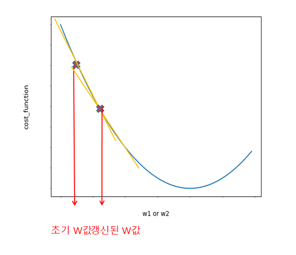
Gradient Decent는 Cost Function을 W에 애해 편미분하면 현재 W위치에서의 접선의 기울기와 같다.
이러한 W값에서 어떤 음수만큼 빼주게 되어 더하게 된다.
\(W(update)=w-a\frac{\partial f_c(x)}{\partial W}\)
즉 W값이 점점 커지면서 새롭게 갱신된 W에 대해서 위와같은 공식을 반복적으로 적용한다.
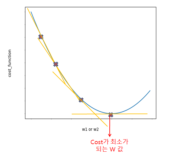
주의해야 할 점은 a(학습률 파라미터 = Learning Rate)를 적절한 값으로 설정해줘야 한다는 것이다.
학습률 파라미터가 너무 작은 값이면 최적의 w를 찾아가는데 너무 오래 걸릴 가능성이 크고, 너무 크면 최적의 지점을 건너뛰어 버리고 발산해 버릴 수 있다.

계속하여 W를 갱신하여 Cost값이 최소가 되는(미분값이 0 인) 곳을 찾는다.

Gradinet 와 Normal Eq 비교
정규방정식(Normal equation 혹은 경사하강법(Gradient Decent)은 통계학에서 선형 회귀상에서 알지 못하는 값(parameter)를 예측하기 위한 방법론이다.
경사 하강법이 수학적 최적화 알고리즘으로서 적절한 학습비율(learning rate)를 설정해야하고 많은 연산량이 필요하지만 아무리 많은 피쳐가 존재하더라도 일정한 시간 내에 해법을 찾는 것이 가능
정규방정식에는 적절한 학습비율(learning rate)를 설정이 없다는 장점이 있다. 하지만 정규방정식은 행렬 연산에 기반하기 때문에 피쳐의 개수가 엄청나게 많을 경우 연산이 느려지는 것을 피할 수 없다. 그러므로 예측 알고리즘을 선택할 때 있어 피쳐의 개수에 따라 알맞은 것을 선택하여야 한다.

Gradient Descent를 위한 실제 미분 유도

앞으로 많이 사용하게 될 공식을 실제로 미분으로서 유도하는 과정을 가져보자.
Activation Function: a = \(\sigma(z) , Sigmoid Function\)
Loss Function:
(1) MSE: \(M = \frac{1}{2} (y - \sigma(z))^2\)
(2) Cross Entrophy: \(J = -{yln(\sigma(z)) + (1-y)ln(1-\sigma(z))}\)
위와같은 가정을 하였을때 Loss Function을 각각 미분을 해보자.
MSE

$${1 \over 2}{(y - \sigma(z))^2 \over dz}$$

$$= -(y - \sigma(z))(\sigma(z))\prime$$

$$= -(y - \sigma(z))\sigma(z)(1-\sigma(z))$$

Cross Entrophy

$${dJ \over dz} = {dJ \over da}{da \over dz}$$

$${dJ \over da} = -{y \over a} + ({1-y \over 1-a}) ({1-a \over da})$$

$$= -{y \over \sigma(z)}-({1-y \over 1-\sigma(z)})$$

$${da \over dz} = \sigma(z)(1-\sigma(z))$$

$${dJ \over dz} = \left\{ \sigma(z)(1-\sigma(z)) \right\} \left\{-{y \over \sigma(z)}-({1-y \over 1-\sigma(z)})\right\}$$

$$= -{y(1-\sigma(z))-\sigma(z)(1-y)}$$

$$= -(y-y\sigma(z)-\sigma(z)+y\sigma(z)))$$

$$= \sigma(z)-y$$

Gradient Descent 구현

Gradient Descent를 구현하기 위해서는 실제 함수의 기울기를 구할 수 있어야 한다.
실제 함수의 기울기를 알기 위해서는 실제 함수의 미분값을 구하면 된다.

함수 미분

#미분 - Parameter: f(함수),x(input_value)
def numerical_gradient(f,x):
    h = 1e-4
    grad = np.zeros_like(x)
    
    for idx in range(x.size):
        
        tmp_val = x[idx]
        
        x[idx] = tmp_val + h
        fxh1 = f(x)
        
        x[idx] = tmp_val - h
        fxh2 = f(x)
        
        grad[idx] = (fxh1-fxh2) /(2*h)
        x[idx] = tmp_val
    
    return grad

함수 미분을 활용하여 GradientDescent를 구현하면 아래와 같다.
Gradient Descent Parameter

Parameter	의미
f	해당 함수
init_x	Input Value
lr	Learning Rate
step_num	반복횟수

Gradient Descent Code

#GradientDescent
def gradient_descent(f,init_x,lr=0.01,step_num=100):
    x=init_x
    
    for i in range(step_num):
        grad = numerical_gradient(f,x)
        x = x-lr*grad
    return x

Gradient Descent를 활용하여 기울기의 변화를 살펴보는 코드이다.
plot_gradient_descent는 x_history라는 변수를 추가하여 실제 x값의 변화를 저장해놓는 parameter이다.

#GradientDescent 예시
#함수선언
def function_2(x):
    return x[0]**2 + x[1]**2

#그리기 위한 Gradient_Descent
#x_history를 통하여 값의 변화를 저장
def plot_gradient_descent(f, init_x, lr=0.01, step_num=100):
    x = init_x
    x_history = []

    for i in range(step_num):
        x_history.append( x.copy() )

        grad = numerical_gradient(f, x)
        x -= lr * grad

    return x, np.array(x_history)

init_x = np.array([-3.0, 4.0])    

lr = 0.1
step_num = 20
x, x_history = plot_gradient_descent(function_2, init_x, lr=lr, step_num=step_num)

plt.plot( [-5, 5], [0,0], '--b')
plt.plot( [0,0], [-5, 5], '--b')
plt.plot(x_history[:,0], x_history[:,1], 'o')

plt.xlim(-3.5, 3.5)
plt.ylim(-4.5, 4.5)
plt.xlabel("X0")
plt.ylabel("X1")
plt.show()

실제 결과

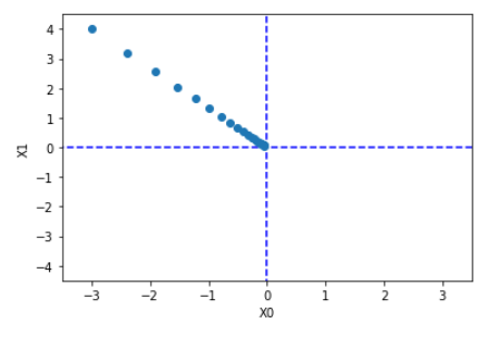
Gradient Descent는 Normal Equation에 비해 장점이 많지만 Learning Rate를 직접 선언해야 하는 단점이 생긴다.
아래 코드는 Learning Rate값을 너무 크거나 작은 경우를 보여준다.
1)Learning Rate이 매우 큰 경우(발산)

#1. 학습률이 매우 큰 예(발산)
init_x = np.array([-3.0,4.0])
print(gradient_descent(function_2,init_x = init_x, lr=10.0, step_num=100)) #[-2.58983747e+13 -1.29524862e+12]

2)Learning Rate이 매우 작은 경우(수렴 X)

#2. 학습률이 매우 작은 예(수렴X)
init_x = np.array([-3.0,4.0])
print(gradient_descent(function_2,init_x = init_x, lr=1e-10, step_num=100)) #[-2.99999994  3.99999992]

Two Layer Network

GradientDescent를 활용하기 위한 2층 Layer를 선언하는 과정이다.
Two Layer Network Method

Method	의미
__init__	Parameter 초기값 설정
predict	예측값(Softmax활용)
loss	Loss Function(Cross Entrophy)
accuracy	정확도(Output이 softmax이므로 argmax활용)
numerical_gradien	미분
gradient	Gradient Descent
cross_entropy_error	Cross Entrophy

Two Layer Network Code

#2층 Layer 선언
class TwoLayerNet:

    #Parameter 초기화
    def __init__(self, input_size, hidden_size, output_size, weight_init_std=0.01):
        # 가중치 초기화
        self.params = {}
        self.params['W1'] = weight_init_std * np.random.randn(input_size, hidden_size)
        self.params['b1'] = np.zeros(hidden_size)
        self.params['W2'] = weight_init_std * np.random.randn(hidden_size, output_size)
        self.params['b2'] = np.zeros(output_size)

    #예측값
    def predict(self, x):
        W1, W2 = self.params['W1'], self.params['W2']
        b1, b2 = self.params['b1'], self.params['b2']
    
        a1 = np.dot(x, W1) + b1
        z1 = sigmoid(a1)
        a2 = np.dot(z1, W2) + b2
        y = softmax(a2)
        
        return y
        
    # x : 입력 데이터, t : 정답 레이블
    def loss(self, x, t):
        y = self.predict(x)
        
        return cross_entropy_error(y, t)
    
    def accuracy(self, x, t):
        y = self.predict(x)
        y = np.argmax(y, axis=1)
        t = np.argmax(t, axis=1)
        
        accuracy = np.sum(y == t) / float(x.shape[0])
        return accuracy
        
    # x : 입력 데이터, t : 정답 레이블
    def numerical_gradient(self, x, t):
        loss_W = lambda W: self.loss(x, t)
        
        grads = {}
        grads['W1'] = numerical_gradient(loss_W, self.params['W1'])
        grads['b1'] = numerical_gradient(loss_W, self.params['b1'])
        grads['W2'] = numerical_gradient(loss_W, self.params['W2'])
        grads['b2'] = numerical_gradient(loss_W, self.params['b2'])
        
        return grads
        
    def gradient(self, x, t):
        W1, W2 = self.params['W1'], self.params['W2']
        b1, b2 = self.params['b1'], self.params['b2']
        grads = {}
        
        batch_num = x.shape[0]
        
        # forward
        a1 = np.dot(x, W1) + b1
        z1 = sigmoid(a1)
        a2 = np.dot(z1, W2) + b2
        y = softmax(a2)
        
        # backward
        dy = (y - t) / batch_num
        grads['W2'] = np.dot(z1.T, dy)
        grads['b2'] = np.sum(dy, axis=0)
        
        da1 = np.dot(dy, W2.T)
        dz1 = sigmoid_grad(a1) * da1
        grads['W1'] = np.dot(x.T, dz1)
        grads['b1'] = np.sum(dz1, axis=0)

        return grads
    
    def cross_entropy_error(y, t):
        if y.ndim == 1:
            t = t.reshape(1, t.size)
            y = y.reshape(1, y.size)
        
        # 훈련 데이터가 원-핫 벡터라면 정답 레이블의 인덱스로 반환
        if t.size == y.size:
            t = t.argmax(axis=1)
             
        batch_size = y.shape[0]
        return -np.sum(np.log(y[np.arange(batch_size), t] + 1e-7)) / batch_size

Activation Function 선언

#사용할 함수 선언
def sigmoid(x):
    return 1 / (1 + np.exp(-x))    


def sigmoid_grad(x):
    return (1.0 - sigmoid(x)) * sigmoid(x)

def softmax(x):
    if x.ndim == 2:
        x = x.T
        x = x - np.max(x, axis=0)
        y = np.exp(x) / np.sum(np.exp(x), axis=0)
        return y.T 

    x = x - np.max(x) # 오버플로 대책
    return np.exp(x) / np.sum(np.exp(x))

def cross_entropy_error(y, t):
    if y.ndim == 1:
        t = t.reshape(1, t.size)
        y = y.reshape(1, y.size)
        
    # 훈련 데이터가 원-핫 벡터라면 정답 레이블의 인덱스로 반환
    if t.size == y.size:
        t = t.argmax(axis=1)
             
    batch_size = y.shape[0]
    return -np.sum(np.log(y[np.arange(batch_size), t] + 1e-7)) / batch_size

Two Layer Network 구현

이전 NerualNetwork (1) Basic & Activation Function에서는 Model을 만들지 못하여 Pickle로 구현되어있는 Model을 가져와서 사용하였다.
하지만 이제 Optimazation까지 구현하였으므로 실제 Model을 선언하고 Weight를 Update하는 Code를 구현하였다.

# coding: utf-8
import sys, os
sys.path.append(os.pardir)  # 부모 디렉터리의 파일을 가져올 수 있도록 설정
import numpy as np
import matplotlib.pyplot as plt
from dataset.mnist import load_mnist

# 데이터 읽기
(x_train, t_train), (x_test, t_test) = load_mnist(normalize=True, one_hot_label=True)

network = TwoLayerNet(input_size=784, hidden_size=50, output_size=10)

# 하이퍼파라미터
iters_num = 10000  # 반복 횟수를 적절히 설정한다.
train_size = x_train.shape[0]
batch_size = 100   # 미니배치 크기
learning_rate = 0.1

train_loss_list = []
train_acc_list = []
test_acc_list = []

# 1에폭당 반복 수
iter_per_epoch = max(train_size / batch_size, 1)

for i in range(iters_num):
    # 미니배치 획득
    batch_mask = np.random.choice(train_size, batch_size)
    x_batch = x_train[batch_mask]
    t_batch = t_train[batch_mask]
    
    # 기울기 계산
    #grad = network.numerical_gradient(x_batch, t_batch)
    grad = network.v(x_batch, t_batch)
    
    # 매개변수 갱신
    for key in ('W1', 'b1', 'W2', 'b2'):
        network.params[key] -= learning_rate * grad[key]
    
    # 학습 경과 기록
    loss = network.loss(x_batch, t_batch)
    train_loss_list.append(loss)
    
    # 1에폭당 정확도 계산
    if i % iter_per_epoch == 0:
        train_acc = network.accuracy(x_train, t_train)
        test_acc = network.accuracy(x_test, t_test)
        train_acc_list.append(train_acc)
        test_acc_list.append(test_acc)
        print("train acc, test acc | " + str(train_acc) + ", " + str(test_acc))

# 그래프 그리기
markers = {'train': 'o', 'test': 's'}
x = np.arange(len(train_acc_list))
plt.plot(x, train_acc_list, label='train acc')
plt.plot(x, test_acc_list, label='test acc', linestyle='--')
plt.xlabel("epochs")
plt.ylabel("accuracy")
plt.ylim(0, 1.0)
plt.legend(loc='lower right')
plt.show()

train acc, test acc | 0.09871666666666666, 0.098
train acc, test acc | 0.78615, 0.793
train acc, test acc | 0.8761666666666666, 0.8794
train acc, test acc | 0.8976, 0.9008
train acc, test acc | 0.9065, 0.911
train acc, test acc | 0.9135333333333333, 0.9183
train acc, test acc | 0.91925, 0.9208
train acc, test acc | 0.9226166666666666, 0.9246
train acc, test acc | 0.92715, 0.9289
train acc, test acc | 0.9302666666666667, 0.9311
train acc, test acc | 0.9331, 0.9328
train acc, test acc | 0.9365666666666667, 0.9369
train acc, test acc | 0.9385833333333333, 0.9377
train acc, test acc | 0.9415833333333333, 0.9412
train acc, test acc | 0.9433, 0.9408
train acc, test acc | 0.9450666666666667, 0.944
train acc, test acc | 0.9460833333333334, 0.9454

구현 결과 그래프로 확인

---

참조: 원본코드
참조: Chanwoo Timothy Lee Youtube
참조: 나무위키
참조: 밑바닥부터 시작하는 딥러닝
문제가 있거나 궁금한 점이 있으면 wjddyd66@naver.com으로 Mail을 남겨주세요.