Ch7.Ensemble Learning and Random Forest

Ensemble Learning and Random Forest

Ensemble Learning이란 여러개의 약 분류기(Weak Classifier)를 결합하여 강 분류기(Strong Classifier)를 만드는 것 이다. 이러한 기법으로서 Model의 정확성이 향상되는 방법이다.

Ensemble Learning기법으로서 배깅, 부스팅, 스태킹 등 인기있는 앙상블 방법이 존재하게 된다.

또한 Randoem Forest는 Decision Tree를 Ensemble기법을 사용하여 Randoem Forest으로서 구성하게 된다.

이번장에 대한 자세한 이론은 Post한 적이 없으므로, 이론과 Code로서 자세히 알아보도록 한다.

Setup

실제 Project를 진행하기 앞서 사용하고자 하는 Library확인 및 원하는 Version(Python 언어 특성상 Version에 많이 의존하게 된다.)이 설치되어있는지 확인하는 작업이다.
또한, 자주 사용하게 될 Function이나, Directory를 지정하기도 한다.

# Python ≥3.5 is required
import sys
assert sys.version_info >= (3, 5)

# Scikit-Learn ≥0.20 is required
import sklearn
assert sklearn.__version__ >= "0.20"

# Common imports
import numpy as np
import os

# to make this notebook's output stable across runs
np.random.seed(42)

# To plot pretty figures
%matplotlib inline
import matplotlib as mpl
import matplotlib.pyplot as plt
mpl.rc('axes', labelsize=14)
mpl.rc('xtick', labelsize=12)
mpl.rc('ytick', labelsize=12)

# Where to save the figures
PROJECT_ROOT_DIR = "."
CHAPTER_ID = "ensembles"
IMAGES_PATH = os.path.join(PROJECT_ROOT_DIR, "images", CHAPTER_ID)
os.makedirs(IMAGES_PATH, exist_ok=True)

def save_fig(fig_id, tight_layout=True, fig_extension="png", resolution=300):
    path = os.path.join(IMAGES_PATH, fig_id + "." + fig_extension)
    print("Saving figure", fig_id)
    if tight_layout:
        plt.tight_layout()
    plt.savefig(path, format=fig_extension, dpi=resolution)

Voting Classifier

Voting Classifier는 “다수결 분류”를 뜻하는 것으로, 크게 2가지 방법으로 분류할 수 있다.

1. Hard Voting Classifier
여러 모델을 생성하고 그 성과(결과)를 비교한다. 이 때 Classifier의 결과들을 집계하여 가장 많은 표를 얻는 클래스를 최종 예측값으로 정하는 것을 Hard Voting Classifier라고 한다.
사진 참조: nonmeyet 블로그

• \(Num(p(i_1|x)) = 3\)
• \(Num(p(i_2|x)) = 1\)
• \(Argmax(Num(p(i_1|x)), Num(p(i_2|x))) = 1 => \text{Ensemble's prediction: 1}\)

2. Soft Voting Classifier
Ensemble에 사용되는 모든 Classifier의 확률을 예측할 수 있을 때 사용한다. 각 분류기의 Prediction의 Probability을 평균 내어 확률이 가장 높은 Class로 예측하게 된다.(가중치 투표)
사진 참조: nonmeyet 블로그

• \(p(i_1|x)) = \frac{0.9+0.8+0.3+0.4}{4}=0.6\)
• \(p(i_2|x)) = \frac{0.1+0.2+0.7+0.6}{4}=0.4\)
• \(Argmax(p(i_1|x), p(i_2|x)) = 1 => \text{Ensemble's prediction: 1}\)

Sklearn Voting Classifier

• Classifier1: Logistic Regression
• Classifier2: RandomForest Classifier
• Classifier3: SVM
• Method of Voting: Hard & Soft

from sklearn.model_selection import train_test_split
from sklearn.datasets import make_moons
from sklearn.metrics import accuracy_score

# Dataset
X, y = make_moons(n_samples=500, noise=0.30, random_state=42)
X_train, X_test, y_train, y_test = train_test_split(X, y, random_state=42)

# Classifier
from sklearn.ensemble import RandomForestClassifier
from sklearn.ensemble import VotingClassifier
from sklearn.linear_model import LogisticRegression
from sklearn.svm import SVC

log_clf = LogisticRegression(solver="lbfgs", random_state=42)
rnd_clf = RandomForestClassifier(n_estimators=100, random_state=42)
svm_clf = SVC(gamma="scale", random_state=42)

print('Classifier')
for clf in (log_clf, rnd_clf, svm_clf):
    clf.fit(X_train, y_train)
    y_pred = clf.predict(X_test)
    print(clf.__class__.__name__, accuracy_score(y_test, y_pred))
    

# Hard Voting Classifier
print('\n\nHard Voting')
voting_clf = VotingClassifier(
    estimators=[('lr', log_clf), ('rf', rnd_clf), ('svc', svm_clf)],
    voting='hard')

voting_clf.fit(X_train, y_train)
y_pred = voting_clf.predict(X_test)
print(voting_clf.__class__.__name__, accuracy_score(y_test, y_pred))

# Soft Voting Classifier
# SVM => Probability
svm_clf = SVC(gamma="scale", probability=True, random_state=42)

print('\n\nSoft Voting')
voting_clf = VotingClassifier(
    estimators=[('lr', log_clf), ('rf', rnd_clf), ('svc', svm_clf)],
    voting='soft')

voting_clf.fit(X_train, y_train)
y_pred = voting_clf.predict(X_test)
print(voting_clf.__class__.__name__, accuracy_score(y_test, y_pred))

Classifier
LogisticRegression 0.864
RandomForestClassifier 0.896
SVC 0.896


Hard Voting
VotingClassifier 0.912


Soft Voting
VotingClassifier 0.92

Bagging & Pasting

Bagging은 Bootstrap Aggregation의 약자이다. Bagging은 Sample을 여러 번 뽑아(Bootstrap) 각 모델을 학습시켜 결과물을 집계(Aggregration)하는 방법이다.

Pasting과 Bagging은 비슷하지만, Bagging은 Bootstrap시 중복을 허용하지 않고, Pasting은 중복을 허용하는 방법이다.

Bagging Model

사진 참조: swallow 블로그

Bias and Variance Trade off를 살펴보게 되면 Model의 Variance를 줄이는 방법은 Dataset을 더 많이 모으는 것 이다.

따라서 Bagging or Pasting을 통하여 Dataset을 많이 확보하게 되면, 개별 Classifier Model의 Bias는 증가하게 되나, Bagging Model을 통과하게 되면서 Bias도 줄고 Variance도 줄일 수 있다. (하지만, 원래 Model보다는 Bias는 증가하게 됩니다.)

from sklearn.ensemble import BaggingClassifier
from sklearn.tree import DecisionTreeClassifier
from sklearn.metrics import accuracy_score
from matplotlib.colors import ListedColormap

# Decision Tree
tree_clf = DecisionTreeClassifier(random_state=42)
tree_clf.fit(X_train, y_train)
y_pred_tree = tree_clf.predict(X_test)
print('Accuracy of Decision Tree: ',accuracy_score(y_test, y_pred_tree))

# Bagging(500 Decision Tree => Ensemble)
bag_clf = BaggingClassifier(
    DecisionTreeClassifier(random_state=42), n_estimators=500,
    max_samples=100, bootstrap=True, random_state=42)
bag_clf.fit(X_train, y_train)
y_pred = bag_clf.predict(X_test)
print('Accuracy of Bagging: ',accuracy_score(y_test, y_pred))

# Visualization
def plot_decision_boundary(clf, X, y, axes=[-1.5, 2.45, -1, 1.5], alpha=0.5, contour=True):
    x1s = np.linspace(axes[0], axes[1], 100)
    x2s = np.linspace(axes[2], axes[3], 100)
    x1, x2 = np.meshgrid(x1s, x2s)
    X_new = np.c_[x1.ravel(), x2.ravel()]
    y_pred = clf.predict(X_new).reshape(x1.shape)
    custom_cmap = ListedColormap(['#fafab0','#9898ff','#a0faa0'])
    plt.contourf(x1, x2, y_pred, alpha=0.3, cmap=custom_cmap)
    if contour:
        custom_cmap2 = ListedColormap(['#7d7d58','#4c4c7f','#507d50'])
        plt.contour(x1, x2, y_pred, cmap=custom_cmap2, alpha=0.8)
    plt.plot(X[:, 0][y==0], X[:, 1][y==0], "yo", alpha=alpha)
    plt.plot(X[:, 0][y==1], X[:, 1][y==1], "bs", alpha=alpha)
    plt.axis(axes)
    plt.xlabel(r"$x_1$", fontsize=18)
    plt.ylabel(r"$x_2$", fontsize=18, rotation=0)
    
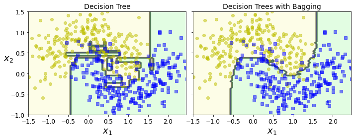
fix, axes = plt.subplots(ncols=2, figsize=(10,4), sharey=True)
plt.sca(axes[0])
plot_decision_boundary(tree_clf, X, y)
plt.title("Decision Tree", fontsize=14)
plt.sca(axes[1])
plot_decision_boundary(bag_clf, X, y)
plt.title("Decision Trees with Bagging", fontsize=14)
plt.ylabel("")
save_fig("decision_tree_without_and_with_bagging_plot")
plt.show()

Accuracy of Decision Tree:  0.856
Accuracy of Bagging:  0.904

Random Forest

Random Forest는 Decision Tree를 개별 모형으로 사용하는 방법이다.

즉, Randoem Forest는 데이터의 특징 차원의 일부만 선택하여 만든 여러개의 Decision Tree를 하나의 Node로서 Tree로 구성하는 것 이다. 간단한 예시로서 살펴보면 다음과 같다.

Algorithm

1. 주어진 Feature에서 일부만 무작위로 Sampling을 한다.
   • Method: Bagging or Pasting
   • Num of Feature: User Select => 전체 Feature에서 몇개의 Feature를 사용할 지는 사용자가 정해야 하며, Model 성능에 영향을 미친다.
2. 주어진 Feature로서 Decision Tree를 생성하게 되고, 이 중 가장 중요한 Feature를 선택하게 된다.
3. 주어진 Decision Tree의 개수만큼 1~2를 수행하게 된다.
4. 3에서의 Feature를 고려하여 하나의 큰 Tree를 만들게 된다.

이러한 방법으로 인하여 모든 요소를 Combination으로서 고려할 수 있고, 이러한 Ensemble방법으로 인하여 성능이 향상되는 것을 기대하는 방법이다.

또한 이렇나 Randoem Forest을 방법을 극단적으로서 표현한 것이 Extremely Randomized Tree이다.

사진 출처: medium.com

Sklearn Random Forest

from sklearn.ensemble import RandomForestClassifier

rnd_clf = RandomForestClassifier(n_estimators=500, max_leaf_nodes=16, random_state=42)
rnd_clf.fit(X_train, y_train)

y_pred_rf = rnd_clf.predict(X_test)

print('Accuracy of Random Forest: ',np.sum(y_pred == y_pred_rf) / len(y_pred))  # almost identical predictions

Accuracy of Random Forest:  0.976

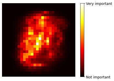
Feature Importance
Decision Tree를 사용하게 되면, Feature의 중요도를 결정할 수 있다.
Decision Tree는 결국 Information Gain이 많은 곳으로 Feature를 결정하게 된다. 이러한 경우 Node와 Parent의 Information Gain차이로 인하여 Feature의 Importance를 측정할 수 있다.

또한, 각각의 Feature가 Root Node가 되는 경우, Tree의 복잡도에 따라서 이 Feature의 중요도를 설명할 수도 있을 것 이다.(중요한 변수가 Root로 오는 경우에 Tree의 복잡도는 줄어들 것 이다.)

현재 Sklearn Randoem Forest의 Feature Importance의 경우에는 1번째로서 Metric을 설정하고 Feature Importance를 결정하게 된다.

from sklearn.datasets import fetch_openml
# Dataset
mnist = fetch_openml('mnist_784', version=1)
mnist.target = mnist.target.astype(np.uint8)

# Model - Random Forest
rnd_clf = RandomForestClassifier(n_estimators=100, random_state=42)
rnd_clf.fit(mnist["data"], mnist["target"])

RandomForestClassifier(bootstrap=True, ccp_alpha=0.0, class_weight=None,
                       criterion='gini', max_depth=None, max_features='auto',
                       max_leaf_nodes=None, max_samples=None,
                       min_impurity_decrease=0.0, min_impurity_split=None,
                       min_samples_leaf=1, min_samples_split=2,
                       min_weight_fraction_leaf=0.0, n_estimators=100,
                       n_jobs=None, oob_score=False, random_state=42, verbose=0,
                       warm_start=False)

# Visualization
def plot_digit(data):
    image = data.reshape(28, 28)
    plt.imshow(image, cmap = mpl.cm.hot,
               interpolation="nearest")
    plt.axis("off")
    
plot_digit(rnd_clf.feature_importances_)

cbar = plt.colorbar(ticks=[rnd_clf.feature_importances_.min(), rnd_clf.feature_importances_.max()])
cbar.ax.set_yticklabels(['Not important', 'Very important'])

save_fig("mnist_feature_importance_plot")
plt.show()

Boosting

(Boosting의 내용은 bkshin 블로그에 정말 잘 정리되어 있어서 그대로 가져오게 되었습니다.)

Boosting은 가중치를 활용하여 약 분류기를 강 분류기로 만드는 방법 입니다. Bagging은 Decision Tree1과 Decision Tree2가 서로 독립적으로 결과를 예측한다.
여러 개의 독립적인 Decision Tree가 가각 값을 예측한 뒤, 그 결과 값을 집계해 최종 결과 값을 예측하는 방식이다.
하지만 Boosting은 Model간 보안을 해 나가는 방식이다. 처음 Model이 예측을 하면 그 예측 결과에 따라 데이터에 가중치가 부여되고, 부여된 가중치가 다음 모델에 영향을 준다. 잘못 분류된 데이터에 집중하여 새로운 분류 규직은 만드는 단계를 반복한다. 아래 그림을 참조하면 다음과 같다.

사진 출처: bkshin 블로그

+와-로 구성된 데이터셋을 분류하는 문제이다.

D1에서는 2/5 지점을 횡단하는 구분선으로 데이터를 나누었다. 하지만 위쪽의 +는 잘못 분류가 되었고, 아래쪽의 두 -도 잘못 분류되었다. 잘못 분류가 된 데이터의 가중치는 높이고, 잘 분류된 데이터는 가중치를 낮춘다.

D2를 보면 D1에서 잘 분류된 데이터는 크기가 작아졌고(가중치가 낮아졌고), 잘못 분류된 데이터는 크기가 커졌다.(가중치가 커졌다.) 분류가 잘못된 데이터에 가중치를 부여해주는 이유는 다음 모델에서 더 집중해 분류하기 위함이다. D2에서는 오른쪽 세 개의 -가 잘못 분류 되었다.

Boosting기법은 결국 앞선 Classifier에서 잘 분류한 Dataset에는 덜 가중치를 주고, 잘못 분류한 Dataset에는 가중치를 더 분류하여 점점 더 잘 Classifier하게 Model을 구성하는 방식이다.

Boosting vs Bagging

사진 출처: bkshin 블로그

• Bagging: 각각의 독립된 Classifier Model을 병렬적으로 학습하여 Voting하는 방식
• Boosting: Classifier Model을 직렬적으로 학습하여, Data의 가중치를 변경해가면서 학습

Boosting은 Bagging에 비해 Error가 적으나, Overfitting이 될 가능성이 높고 학습 속도가 느리다.(High Variance) Classifier의 성능 자체가 낮다면 Boosting을 사용(High Bias)하고, Overfitting이 문제이면 Bagging을 사용하는 것이 적당한 방법일 것 이다. (결국 ML에서의 문제인 Bias and Variance Trade Off문제에서 사용자가 선택하는 문제이다.)

Formula

Formula인 경우 데이터 사이언스 스쿨을 참조 하였습니다.

Boosting
Classifier의 집합을 C(commitee)라고 표현하고 약 분류기(weak classifier)로서 표현한다면 m개의 Weak classifier를 포함하는 Commitee는 \(C_m\)으로서 표현한다.

위와 같이 정의한다면 Boosting을 다음과 같이 정의할 수 있다.

$$ \begin{gather} C_1 = \{ k_1 \} \\ C_2 = C_1 \cup k_2 = \{ k_1, k_2 \} \\ C_3 = C_2 \cup k_3 = \{ k_1, k_2, k_3 \} \\ \vdots \\ C_m = C_{m-1} \cup k_m = \{ k_1, k_2, ..., k_m \} \end{gather} $$

Boosting방법은 최종적으로 각각의 weak classifier를 가중치를 곱하여 판별하게 된다. 즉, 최종적인 판단은 다음과 같이 나타낼 수 있다.(Label = -1 or 1인 Binary Classifier의 경우)

$$ \begin{gather} y = -1 \text{ or } 1 \\ C_{m}(x_i) = \text{sign} \left( \alpha_1k_1(x_i) + \cdots + \alpha_{m}k_{m}(x_i) \right) \end{gather} $$

AdaBoost
AdaBoost라는 이름은 적응 부스트(adaptive boost)라는 용어에서 나왔다. Adaboost는 Commitee에 넣을 개별 모형 \(k_m\)을 선별하는 방법으로 학습 데이터의 집합의 i번째 데이터에 가중치 \(w_i\)를 주고 분류 모형이 틀리게 예측한 데이터의 가중치를 합한 값을 Loss로 사용한다. 이 손실함수를 최소화하는 모형이 \(k_m\) 으로선택된다.

즉, AdaBoost는 크게 2가지를 고려하여 구성된다.

1. 전체 판별기 \(C_m\)안의 각각의 Weak Classifier(\(k_m\))의 중요도(\(\alpha_m\))를 설정하여야 한다.
2.Weak Classifier(\(k_m\))안에서 각각의 데이터에 대한 가중치를 구해야 한다.(\(w_{m,i}\))

Loss Function
먼저 AdaBoost의 LossFunction을 살펴보면 다음과 같다.

$$L_m = \sum_{i=1}^{N}w_{m,i}I(k_m(x_i) \neq y_i)$$

$$ I= \begin{cases} 1, & \mbox{if } k_m(x_i) \neq y_i \\ 0, & \mbox{if } k_m(x_i) = y_i \end{cases} $$

\(\alpha_m\)
위의 Loss를 활용하여 \(\alpha_m\)의 값은 다음과 같이 정의된다.

$$\epsilon_m = \dfrac{\sum_{i=1}^N w_{m,i} I\left(k_m(x_i) \neq y_i\right)}{\sum_{i=1}^N w_{m,i}}$$

$$\alpha_m = \frac{1}{2}\log\left( \frac{1 - \epsilon_m}{\epsilon_m}\right)$$

위의 식을 살펴보게 되면, 각각의 Weak Classifier에 대한 Weight는 Classifier의 Loss가 적을수록 큰 값을 할당하는 것을 알 수 있다.

\(w_{m,i}\)

$$ w_{m,i} = w_{m-1,i} \exp (-y_iC_{m-1}) = \begin{cases} w_{m-1,i}e^{-1} & \text{ if } C_{m-1} = y_i\\ w_{m-1,i}e & \text{ if } C_{m-1} \neq y_i \end{cases} $$

$$w_{m,i} = \frac{w_{m,i}}{\sum_{i=1}^N w_{m,i}} \text{ Normalization}$$

위의 식을 살펴보게 되면, w는 0~1사이의 값을 가지는 것을 확인할 수 있다. 또한, 틀린문제에 대해서는 weight가 증가되고, 맞춘 문제에 대해서는 weight가 감소되는 것을 알 수 있다. (위의 식이 Converge하다는 것을 자세히 알고 싶으신 분은 데이터 사이언스 스쿨를 참조하시면 되겠습니다.)

Regularization
AdaBoost도 또한 Weak Classifier(\(k_m\))의 개수나 각각의 Weak Classifier의 Complexity에 따라서 Overfitting이 발생할 수 있다.
이에 관하여 Overfitting을 방지하는 식은 다음과 같다.

$$C_m = C_{m-1} + \mu \alpha_m k_m$$

즉 \(\alpha\)가 1보다 작을경우 새로운 commitee의 가중치를 낮춰 Overfitting을 방지하는 것 이다.

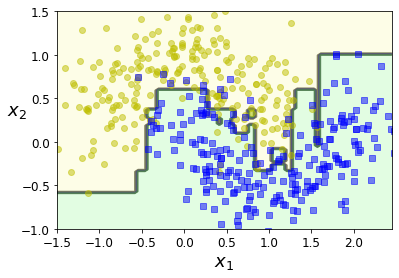
Sklearn AdaBoost

• weak classifier: Decision Tree with max_depth=1
• number of weak classifier: 200
• learning rate: 0.5

from sklearn.ensemble import AdaBoostClassifier

ada_clf = AdaBoostClassifier(
    DecisionTreeClassifier(max_depth=1), n_estimators=200,
    algorithm="SAMME.R", learning_rate=0.5, random_state=42)
ada_clf.fit(X_train, y_train)

plot_decision_boundary(ada_clf, X, y)

AdaBoost + Regularization

m = len(X_train)

fix, axes = plt.subplots(ncols=2, figsize=(10,4), sharey=True)
for subplot, learning_rate in ((0, 1), (1, 0.5)):
    sample_weights = np.ones(m)
    plt.sca(axes[subplot])
    for i in range(5):
        svm_clf = SVC(kernel="rbf", C=0.05, gamma="scale", random_state=42)
        svm_clf.fit(X_train, y_train, sample_weight=sample_weights)
        y_pred = svm_clf.predict(X_train)
        sample_weights[y_pred != y_train] *= (1 + learning_rate)
        plot_decision_boundary(svm_clf, X, y, alpha=0.2)
        plt.title("learning_rate = {}".format(learning_rate), fontsize=16)
    if subplot == 0:
        plt.text(-0.7, -0.65, "1", fontsize=14)
        plt.text(-0.6, -0.10, "2", fontsize=14)
        plt.text(-0.5,  0.10, "3", fontsize=14)
        plt.text(-0.4,  0.55, "4", fontsize=14)
        plt.text(-0.3,  0.90, "5", fontsize=14)
    else:
        plt.ylabel("")

save_fig("boosting_plot")
plt.show()

Gradient Boosting
Gradient Boosting은 변분법(calculus of variations)를 사용한 모형이다.
먼저 Boosting 방법을 다시 생각하면 다음과 같이 나타낼 수 있다.

$$C_m(x_i) = \sum_{j=1}^m \alpha_j k_j(x_i) = C_{m-1}(x_i) + \alpha_m k_m(x_i)$$

Gradient Boosting모형은 위와 같은 식을 DL과 같이 Loss Function(y,\(=C_{m-1}\))을 최소화 하는 \(k_m\)을 찾는 방법이다.

$$C_{m} = C_{m-1} - \alpha_m \dfrac{\delta L(y, C_{m-1})}{\delta C_{m-1}} = C_{m-1} + \alpha_m k_m$$

Gradient Boosting Model은 다음과 같은 과정을 반복하여 weak classifier(\(k_m\))와 그 가중치(\(\alpha_m\))를 계산한다.

1. \(-\tfrac{\delta L(y, C_m)}{\delta C_m}\)를 목표값으로 개별 Weak classifier(\(k_m\))을 찾는다.
2. \(\left( y - (C_{m-1} + \alpha_m k_m) \right)^2\)를 최소화하는 가중치(\(\alpha_m\))를 찾는다.
3. \(C_m = C_{m-1} + \alpha_m k_m\)를 최종 모형으로 선택한다.

ex) LossFunction = MSE

$$L(y, C_{m-1}) = \dfrac{1}{2}(y - C_{m-1})^2$$

Gradient

$$-\dfrac{dL(y, C_m)}{dC_m} = y - C_{m-1}$$

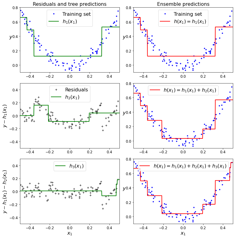
Sklearn Gradient Boosting

• Model: DecisionTreeRegressor
• Num of Model: 3

from sklearn.tree import DecisionTreeRegressor

# Dataset
np.random.seed(42)
X = np.random.rand(100, 1) - 0.5
y = 3*X[:, 0]**2 + 0.05 * np.random.randn(100)

# Model1
tree_reg1 = DecisionTreeRegressor(max_depth=2, random_state=42)
tree_reg1.fit(X, y)

# Model2
y2 = y - tree_reg1.predict(X)
tree_reg2 = DecisionTreeRegressor(max_depth=2, random_state=42)
tree_reg2.fit(X, y2)

# Model3
y3 = y2 - tree_reg2.predict(X)
tree_reg3 = DecisionTreeRegressor(max_depth=2, random_state=42)
tree_reg3.fit(X, y3)

# Visualization
def plot_predictions(regressors, X, y, axes, label=None, style="r-", data_style="b.", data_label=None):
    x1 = np.linspace(axes[0], axes[1], 500)
    y_pred = sum(regressor.predict(x1.reshape(-1, 1)) for regressor in regressors)
    plt.plot(X[:, 0], y, data_style, label=data_label)
    plt.plot(x1, y_pred, style, linewidth=2, label=label)
    if label or data_label:
        plt.legend(loc="upper center", fontsize=16)
    plt.axis(axes)
    
plt.figure(figsize=(11,11))

plt.subplot(321)
plot_predictions([tree_reg1], X, y, axes=[-0.5, 0.5, -0.1, 0.8], label="$h_1(x_1)$", style="g-", data_label="Training set")
plt.ylabel("$y$", fontsize=16, rotation=0)
plt.title("Residuals and tree predictions", fontsize=16)

plt.subplot(322)
plot_predictions([tree_reg1], X, y, axes=[-0.5, 0.5, -0.1, 0.8], label="$h(x_1) = h_1(x_1)$", data_label="Training set")
plt.ylabel("$y$", fontsize=16, rotation=0)
plt.title("Ensemble predictions", fontsize=16)

plt.subplot(323)
plot_predictions([tree_reg2], X, y2, axes=[-0.5, 0.5, -0.5, 0.5], label="$h_2(x_1)$", style="g-", data_style="k+", data_label="Residuals")
plt.ylabel("$y - h_1(x_1)$", fontsize=16)

plt.subplot(324)
plot_predictions([tree_reg1, tree_reg2], X, y, axes=[-0.5, 0.5, -0.1, 0.8], label="$h(x_1) = h_1(x_1) + h_2(x_1)$")
plt.ylabel("$y$", fontsize=16, rotation=0)

plt.subplot(325)
plot_predictions([tree_reg3], X, y3, axes=[-0.5, 0.5, -0.5, 0.5], label="$h_3(x_1)$", style="g-", data_style="k+")
plt.ylabel("$y - h_1(x_1) - h_2(x_1)$", fontsize=16)
plt.xlabel("$x_1$", fontsize=16)

plt.subplot(326)
plot_predictions([tree_reg1, tree_reg2, tree_reg3], X, y, axes=[-0.5, 0.5, -0.1, 0.8], label="$h(x_1) = h_1(x_1) + h_2(x_1) + h_3(x_1)$")
plt.xlabel("$x_1$", fontsize=16)
plt.ylabel("$y$", fontsize=16, rotation=0)

save_fig("gradient_boosting_plot")
plt.show()

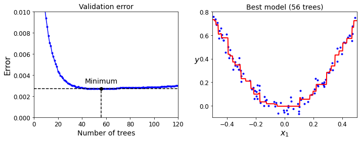
Gradient Boosting with Early stopping
Early Stopping이라는 것은 ML의 Funtion Approximation과 Generalization을 모두 고려하여 Model의 Complexity를 줄이거나, Trainning을 도중에 끊는 방법이다.
즉, Overfitting을 피하기 위한 하나의 방법이다.

아래 Code는 Sklearn에서 GradientBoostingRegressor Model에 Early Stopping을 적용한 것 이다.

Code를 자세히 보면, gbrt_best = GradientBoostingRegressor(max_depth=2, n_estimators=bst_n_estimators, random_state=42)로서 120개의 Boosting Model을 설정하고, Validation Set으로 Validation Loss가 최저인 갯수를 구하게 된다.

import numpy as np
from sklearn.model_selection import train_test_split
from sklearn.metrics import mean_squared_error
from sklearn.ensemble import GradientBoostingRegressor

# Dataset
X_train, X_val, y_train, y_val = train_test_split(X, y, random_state=49)

# Model => Max(Num of Model) = 120
gbrt = GradientBoostingRegressor(max_depth=2, n_estimators=120, random_state=42)
gbrt.fit(X_train, y_train)

# Error List
errors = [mean_squared_error(y_val, y_pred)
          for y_pred in gbrt.staged_predict(X_val)]
bst_n_estimators = np.argmin(errors) + 1

# Model Training
gbrt_best = GradientBoostingRegressor(max_depth=2, n_estimators=bst_n_estimators, random_state=42)
gbrt_best.fit(X_train, y_train)

# Min Error => Best Model with Early Stopping
min_error = np.min(errors)
print("Minimum validation MSE:", min_error)

# Visualization
plt.figure(figsize=(10, 4))

plt.subplot(121)
plt.plot(errors, "b.-")
plt.plot([bst_n_estimators, bst_n_estimators], [0, min_error], "k--")
plt.plot([0, 120], [min_error, min_error], "k--")
plt.plot(bst_n_estimators, min_error, "ko")
plt.text(bst_n_estimators, min_error*1.2, "Minimum", ha="center", fontsize=14)
plt.axis([0, 120, 0, 0.01])
plt.xlabel("Number of trees")
plt.ylabel("Error", fontsize=16)
plt.title("Validation error", fontsize=14)

plt.subplot(122)
plot_predictions([gbrt_best], X, y, axes=[-0.5, 0.5, -0.1, 0.8])
plt.title("Best model (%d trees)" % bst_n_estimators, fontsize=14)
plt.ylabel("$y$", fontsize=16, rotation=0)
plt.xlabel("$x_1$", fontsize=16)

save_fig("early_stopping_gbrt_plot")
plt.show()

Minimum validation MSE: 0.002712853325235463

XGBoost

XGBoost는 Gradient Boosting Model과 비슷하나 다음과 같은 장점이 부각된다.

1. 병렬 처리를 사용하기에 학습과 분류가 빠르다.
2. 유연성이 좋다. 평가 함수를 포함하여 다양한 커스텀 최적화 옵션을 제공한다.
3. Greedy-algorithm을 사용하여 Purning이 가능하다. => Overfitting방지
4. 다른 알고리즘과 연계 활용성이 좋다. 즉, 다른 알고리즘을 붙여서 앙상블 학습이 가능하다.

Gradient Boosting Model이고 또한, Taylor Approximation으로서 1차 미분이 아닌 이차미분까지 사용한다는 점에서 정확도가 향상될 것 이다. 또한, Regularization을 사용하여 Overfitting을 방지하였다.

XGBoost에 대한 자세한 내용은 towardsdatascience을 참조하자. (Gradient Boosting Model과 거의 동일하여 생략. 병렬처리가 어떻게 되는지는 모르겠음)

import xgboost

# XGBoost Model
xgb_reg = xgboost.XGBRegressor(random_state=42)
# eval_set: Validation Dataset
# Early_stopping = 2 => If the error continues to increase during 2 steps, Training Stop
xgb_reg.fit(X_train, y_train,eval_set=[(X_val, y_val)], early_stopping_rounds=2)
y_pred = xgb_reg.predict(X_val)
val_error = mean_squared_error(y_val, y_pred)  # Not shown
print("Validation MSE:", val_error)

[0]	validation_0-rmse:0.22834
Will train until validation_0-rmse hasn't improved in 2 rounds.
[1]	validation_0-rmse:0.16224
[2]	validation_0-rmse:0.11843
[3]	validation_0-rmse:0.08760
[4]	validation_0-rmse:0.06848
[5]	validation_0-rmse:0.05709
[6]	validation_0-rmse:0.05297
[7]	validation_0-rmse:0.05129
[8]	validation_0-rmse:0.05155
[9]	validation_0-rmse:0.05211
Stopping. Best iteration:
[7]	validation_0-rmse:0.05129

Validation MSE: 0.0026308690413069744

---

참조: 원본코드
참조: nonmeyet 블로그
참조: medium.com
참조: bkshin 블로그
참조: 데이터 사이언스 스쿨
참조: towardsdatascience
코드에 문제가 있거나 궁금한 점이 있으면 wjddyd66@naver.com으로 Mail을 남겨주세요.