
Theory11. ICA
현재 Dimension Reduction방법으로 많이 사용되는 것이 SVD, PCA와 AutoEncoder이다.
Dimension Reduction의 방법 중 다른 한 방법으로서 ICA가 있다.
먼저 Code로서 ICA의 Example을 살펴보면 다음과 같다.
ICA Example
1
2
3
4
5
6
7
8
9
10
11
12
13
14
15
16
17
18
19
20
21
22
import pandas as pd
import numpy as np
from scipy import signal
import matplotlib.pyplot as plt

from sklearn.decomposition import FastICA, PCA

np.random.seed(0)  # set seed for reproducible results
n_samples = 2000
time = np.linspace(0, 8, n_samples)

s1 = np.sin(2 * time)  # Signal 1 : sinusoidal signal
s2 = np.sign(np.sin(3 * time))  # Signal 2 : square signal
s3 = signal.sawtooth(2 * np.pi * time)  # Signal 3: sawtooth signal

S = np.c_[s1, s2, s3]
S += 0.2 * np.random.normal(size=S.shape)  # Add noise

S /= S.std(axis=0)  # Standardize data
# Mix data
A = np.array([[1, 1, 1], [0.5, 2, 1.0], [1.5, 1.0, 2.0]])  # Mixing matrix
X = np.dot(S, A.T)  # Generate observations
Low Level ICA
1
2
3
4
5
6
7
8
9
10
11
12
13
14
15
16
17
18
19
20
21
22
23
24
25
26
# compute ICA
ica = FastICA(n_components=3)
S_ = ica.fit_transform(X) # Get the estimated sources
A_ = ica.mixing_ # Get estimated mixing matrix
# compute PCA
pca = PCA(n_components=3)
H = pca.fit_transform(X) # estimate PCA sources
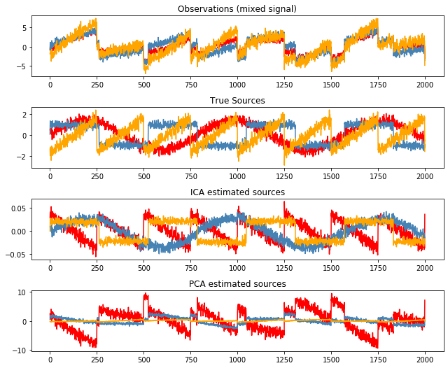
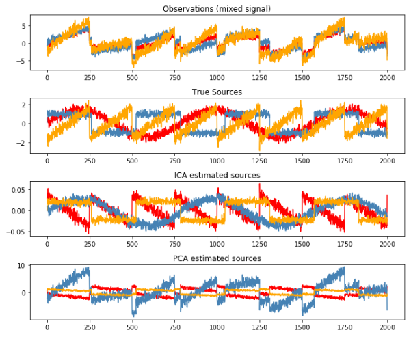
plt.figure(figsize=(9, 9))
models = [X, S, S_,H]
names = ['Observations (mixed signal)',
'True Sources',
'ICA estimated sources',
'PCA estimated sources']
colors = ['red', 'steelblue', 'orange']
for ii, (model, name) in enumerate(zip(models, names), 1):
plt.subplot(5, 1, ii)
plt.title(name)
for sig, color in zip(model.T, colors):
plt.plot(sig, color=color)
plt.tight_layout()
plt.show()
ICA(Independent )
- $X$: Observation Data
- $S$: Source
- $A$: Linear Transformation(Mixing Matrix)
- $W$: Unmixing Matrix
$$X = AS$$
$$S = WX\text{ (}W = A^{-1})$$
즉 우리는 X라는 Signal을 Observation하였을 때 Source Signal의 Linear Tranfomation으로 생각할 수 있다.(Blind Source Separation)
Where it is used
Signal Separation
Remove Artifical Signal in EEG


사진 참조:artifact.html
Assumption
- Source is Independent
- Source is not Gaussian Distribution(or only 1 Souce is GaussianDistribution)
Uncorrelatedness -> Independent(X)
Independent -> Uncorrelatedness(O)
PCA Image
PCA -> 분산이 가장 큰 축으로서 Projection할 수 있다. -> 분산이 최대화 되는 축 -> Correlation을 가장 잘 나타내는 축을 찾는 것 -> Uncorrelatedness라고 설명 가능 -> But not Independent
따라서, ICA라는 것은 PCA보다 더 조건을 많이 주어서 Independent한 신호를 찾는 것 이다.
Preprocessing
1. Centering
$$x = x - \mu$$
Zero mean
2. Whitening
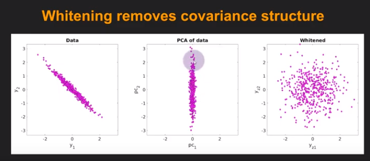
사진 참조: YouTube
각가의 데이터의 분포가 Uncorrlated하고 없게 나타내면서 Same Variance를 같게 하는 과정
$$XX^{T} = EDE^{T}$$
$$\because XX^{T}\text{: Symmetric Matrix}, E: \text{Orthogonal Matrix}, D: \text{Diagonal Matrix, Eigen Value}$$
$$\bar{X} = ED^{-1/2}E^{T}X$$
$$E[\bar{X} \bar{X}^{T}]$$
$$=E[ED^{-1/2}E^{T}X(ED^{-1/2}E^{T}X)^T]$$
$$=E[ED^{-1/2}E^{T}XX^{T}ED^{-1/2}E^T] = I$$
위의 등식을 전에 선언하였던 $X = AS$에 대입하면 다음과 같다.
$$\bar{X} = ED^{-1/2}EAS = \bar{A}S ( \bar{A} = ED^{-1/2}E^{T}A)$$
$$E[\bar{X}\bar{X}^{T}] = \bar{A} E[SS^{T}] \bar{A}^{T} = \bar{A}\bar{A}^{T} = I$$
위의 결과로 인하여 Witening변환을 수행하게 되면 Same Variance를 갖게 되고 추정해야할 A가 Orthogonal Matrix가 되어서 Complexity($n^2 -> n(n-1)/2$)가 준 것을 알 수 있다.
참조($E[SS^{T}] = I$)
$$X = AS = [AC^{-1}][CS] = A^{'}S^{'}$$
$$C = diag(c_1,c_2,...) \text{: Scaling Factor}$$
위와 같이 Scaling Factor를 사용하여 값을 바꾼다고 가정하면, 형태는 같지만, $E[SS^{T}] = I$로 나타낼 수 있기 때문에 위와 같은 조건을 사용할 수 있다.
참조: 자세한 내용
Why not Gaussian Distribution(or only 1 Souce is GaussianDistribution)
Preprocessing -> Centering, Whitening
$X = AS$에서 A는 Orthogonal Matrix 즉, 회전변환 행렬인 것을 알았다.
만약에 Source의 $s_1,s_2$가 Gaussian Distribution이라고 가정하자.
Independent하므로 $p(s_1,s_2) = p(s_1)p(s_2)$가 성립할 것이다.
$$p(s_1,s_2) = \frac{1}{2\pi}exp(-\frac{s_1^2+s_2^2}{2})$$
(Uncorrelated하고 unit variance를 가진다고 가정.)
 우리는 식 $X = AS$에서 A를 Orthogonal Matrix로 정의하였으므로, 위의 그림에서 회전변환을 통하여 X를 추정할 수 있다.
하지만 위의 그림을 어떤 방향으로 돌려도 결국 같은 분포가 나오게 A를 추정할 수 없게 된다.
Nongaussian is Independent
Assumption
- Source is Independent
- Source is not Gaussian Distribution(or only 1 Souce is GaussianDistribution)
Use Central Limit Theore
Central Limit Theore: 동일한 확률분포를 가진 독립 확률변수 n개의 평균의 분포는 n이 적당이 크다면 정규분포에 가까워 진다.
$$y = w^{T}x = w^{T}As = z^{T}s$$
$$w: \text{one of row of Inverse of A}$$
S는 Indepedent Signal이므로 y는 Independent한 확률분포의 Linear Combination이라고 생각할 수 있다.
즉, y는 그 어떤 S보다도 더 Gaussian Distribution에 가깝다.
따라서 우리가 앞으로의 ICA의 Training해야 하는 방향은 $w^{T}$의 값을 변형시켜서 $w^{T}x$의 Maximize Nongaussianity를 수행해야 한다.
ICA = objective function(Maximize Nongaussianity) + optimization algorithm
How to measure Nongaussianty?
NegEntropy
우리는 이제 w를 Nongaussianty에 가깝게 변형시켜야 된다는 것을 알았다.
다음과 같이 Entropy식을 정의하자.
Entropy
$$H(Y) = -\sum_{i}P(Y)logP(Y)$$
A gaussian variable has the largest entropy among all random variables of equal variant
즉, Gausian Variables는 Random Variable에서 가장 큰 Entropy를 가진다.
따라서 우리는 다음과 같이 Negentropy를 정의할 수 있다.
$$J(Y) = H(Y_{gauss}) - H(y)$$
위의 식은 항상 0보다 크게 나올 것이고 Random Variabale이 Gausian Variable일 경우 0이 나오게 될 것이다.
-> 고차 Moment를 이용하여 NegEntropy 추정(M.C. Jones, R.Sibson)
$$J(y) \approx \frac{1}{12}E[y^3]^2 + \frac{1}{48}kurt(y)^2$$
$$kurt(y) = E[y^4]-3(E[y^2])^2$$
=> kurt는 Outlier에 영향을 많이 받는다.
-> A.Hyvarinen
$$J(y) \approx \sum_{1}^{p} k_i [E[G_i (y)] - E[G_y (v)]]^2$$
$$J(Y) \propto [E[G (y)] - E[G (v)]]^2$$
$$k_i: \text{Positive Constants}$$
$$v: \text{Gaussian variable of zero mean and unit variance}$$
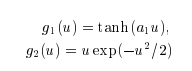
$$y: \text{zerom mean and unit variance}$$
$$G_i: \text{nonquardratic function }$$
$$G_1(u) = -exp(-u^2/2), G_2(u) = \frac{1}{a_1}log cosh a_1 u (1 \le a_1 \le 2)$$
Choosing G that does not grow too fast, one obtains more robust estimation.
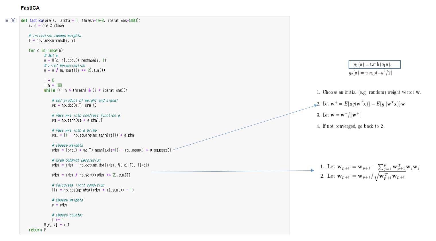
Fast ICA
One Unit
Preprocessing과정을 거쳤으면 다음과 같은 Fast ICA Algorithm을 사용할 수 있다.
$$J(Y) \propto [E[G (y)] - E[G (v)]]^2$$
에서 J(Y)를 최대화 하는 것이 NonGaussianty를 최대화 하는 것 이였다.
$v$는 Gaussian variable of zero mean and unit variance라고 지정하였으므로 NonGaussianty를 최대화 하는 것은 $[E[G (y)]$를 최대화 하는 문제로 바꿔서 생각할 수 있다.
$$y_i = w_i^T x, y=Wx$$
이면 처음 W를 Random하게 Initialization하였다고 생각하자 그렇다면 위의 식은 다시 아래와 같이 변경될 수 있다.
$$\sum_i E[G(y_i)] = \sum_i E[G(w_i^T x)]$$
Preprocessing에서 Centering, Whitening전처리를 통하여 우리는 A가 Orthogonal Matrix라는 결론을 얻었다.
$$A: Orthogonal Matrix -> W=Inverse A = A^{T}$$
$$\therefore W: Orhtogonal Matrix -> ww^T = 1$$
$$w: \text{row vector in Matrix} W$$
위에서 얻은 $ww^T = 1$이라는 조건을 사용하여 $E[G(w^T x)]$의 최대값을 구하기 위하여 Lagrange multiplier를 적용한다.
Lagrange multiplier

$$L(x,y,\lambda) = f(x,y) - \lambda(g(x,y)-c)$$
$$\frac{\partial f}{\partial x} = \lambda \frac{\partial g}{\partial x}$$
$$\frac{\partial f}{\partial y} = \lambda \frac{\partial g}{\partial y}$$
f(x,y): Maximum지점을 찾기 위한 함수, g(x,y) = c는 조건
위의 식에서 구하고자 하는 함수와 조건을 넣으면 다음과 같이 Object Function을 얻을 수 있다.
$$O(w) = E[G(w^T x)] - \beta(w^T w -1)/2$$
$$F(w) = \frac{\partial O(w)}{\partial w} = E[xg(w^T x)] - \beta w = 0$$
$$g(x) = \text{deviative of }G(x)$$
위의 식에서 F(w)가 0이 되도록 w를 Update하면 된다.
Nweton Raphson Method
The Newton-Raphson method (also known as Newton’s method) is a way to quickly find a good approximation for the root of a real-valued function f(x) = 0

$$x_{n+1} = x_{n} - \frac{f(x_n)}{f^{'}(x_n)}$$
위의 식 $F(W) = 0$을 찾기 위하여 Newton Raphson Method를 사용하면 다음과 같다.
$$F(w) = E[xg(w^T x)] - \beta w = 0$$
$$\frac{\partial F(w)}{\partial w}= E[xx^Tg^{'}(w^Tx)] - \beta I$$
$$E[xx^Tg^{'}(w^Tx)] \approx E[xx^T]E[g^{'}(w^Tx)] = E[g^{'}(w^Tx)]I$$
$$\because E[xx^T] = I (\text{ Preprocessing})$$
$$\therefore \frac{\partial F(w)}{\partial w} = E[g^{'}(w^Tx)] - \beta$$
$$\because E[g^{'}(w^Tx)]\text{: Jacobian Matrix -> Diagonal} $$
따라서 위의 식을 사용 하여 Update를 하게 되면 다음과 같다.
$$w <= w - \frac{1}{E[g^{'}(w^Tx)] - \beta}[E[xg(w^T x)] - \beta w]$$
Scalar값 $E[xx^Tg^{‘}(w^Tx)] - \beta$를 곱하게 되면 최종적인 식은 다음과 같다.
$$w <= [E[xg(w^T x)] - E[g^{'}(w^Tx)]]w$$
위에서 Scalar값을 곱하였으니 다시 w를 Normalization하면서 계속해서 0값을 Update한다.
$$w <= w/||w||$$
참조(Jacovian Matrix): explained.ai
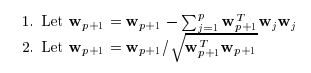
FastICA for several units
W = w 인 상황이 아니라 $W = w_1, w_2, w_3$인 경우는 각각의 w가 Orthogonal하게 Local Minima(왜 w를 Local Minia인 지에 대해서는 Mutual Information에 적용하여 설명하였으나, 생략)를 찾아가야 한다. 즉, 위처럼 One Units로서 계속하여 w를 Update하는 경우 모든 w가 같은 값으로서 수렴될 수 있다.
Gram-Schmidt
Vector의 Component들을 Orthogonal하게 바꾸는 과정이다.
식으로서 표현하면 다음과 같다.
$$u_{k} = v_{k} - \sum_{i=1}^{k-1} proj_{u_j}(v_k)$$
간단히 말하자면 하나의 Vector를 이전 모든 Vector로서 Projection하고 그 값을 없앤다는 의미이다.
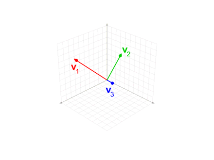
Gram-Schmidt을 사용하게 되면 서로 Orthogonal한 방향으로 겹치는 부분없이 Local Minima를 찾을 수 있게 된다.
Fast ICA Code
Data
1
2
3
4
5
6
7
8
9
10
11
12
13
14
15
16
17
18
# Set a seed for the random number generator for reproducibility
np.random.seed(23)
# Number of samples
ns = np.linspace(0, 200, 1000)
# Source matrix
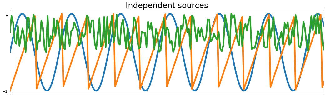
S = np.array([np.sin(ns * 1),
signal.sawtooth(ns * 1.9),
np.random.random(len(ns))]).T
# Mixing matrix
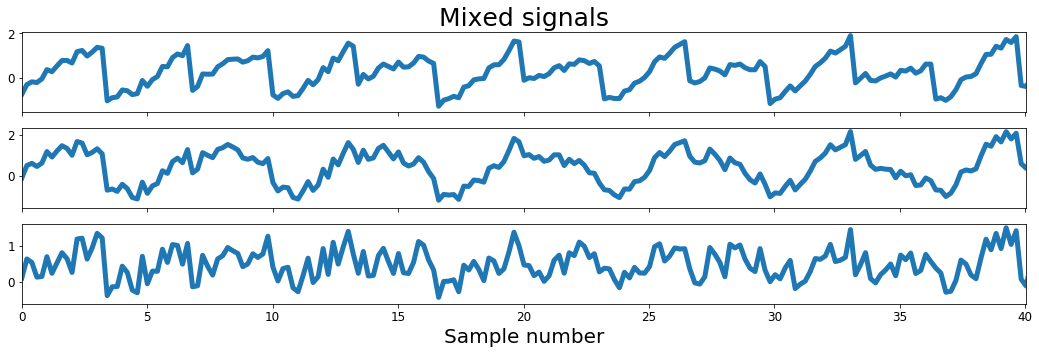
A = np.array([[0.5, 1, 0.2],
[1, 0.5, 0.4],
[0.5, 0.8, 1]])
# Mixed signal matrix
X = S.dot(A).T
DataVisualization
1
2
3
4
5
6
7
8
9
10
11
12
13
14
15
16
17
18
19
20
21
22
23
24
25
# Plot sources & signals
fig, ax = plt.subplots(1, 1, figsize=[18, 5])
ax.plot(ns, S, lw=5)
ax.set_xticks([])
ax.set_yticks([-1, 1])
ax.set_xlim(ns[0], ns[200])
ax.tick_params(labelsize=12)
ax.set_title('Independent sources', fontsize=25)

fig, ax = plt.subplots(3, 1, figsize=[18, 5], sharex=True)
ax[0].plot(ns, X[0], lw=5)
ax[0].set_title('Mixed signals', fontsize=25)
ax[0].tick_params(labelsize=12)

ax[1].plot(ns, X[1], lw=5)
ax[1].tick_params(labelsize=12)
ax[1].set_xlim(ns[0], ns[-1])

ax[2].plot(ns, X[2], lw=5)
ax[2].tick_params(labelsize=12)
ax[2].set_xlim(ns[0], ns[-1])
ax[2].set_xlabel('Sample number', fontsize=20)
ax[2].set_xlim(ns[0], ns[200])

plt.show()
Preprocessing
1
2
3
4
def center(x):
    mean = np.mean(x, axis=1, keepdims=True)
    centered =  x - mean
    return centered, mean
1
2
3
4
5
6
def covariance(x):
    mean = np.mean(x, axis=1, keepdims=True)
    n = np.shape(x)[1] - 1
    m = x - mean

    return (m.dot(m.T))/n
1
2
3
4
5
6
7
8
9
10
11
12
13
14
15
16
17
def whiten(x):
    # Calculate the covariance matrix
    coVarM = covariance(X)

    # Single value decoposition
    U, S, V = np.linalg.svd(coVarM)

    # Calculate diagonal matrix of eigenvalues
    d = np.diag(1.0 / np.sqrt(S))

    # Calculate whitening matrix
    whiteM = np.dot(U, np.dot(d, U.T))

    # Project onto whitening matrix
    Xw = np.dot(whiteM, X)

    return Xw, whiteM
FastICA
위에서 알아본 Algorithm에 적용하면 다음과 같다.
1
2
3
4
5
6
7
8
9
10
11
12
13
14
15
16
17
18
19
20
21
22
23
24
25
26
27
28
29
30
31
32
33
34
35
36
37
38
39
40
41
42
43
def fastIca(pre_X,  alpha = 1, thresh=1e-8, iterations=5000):
    m, n = pre_X.shape

    # Initialize random weights
    W = np.random.rand(m, m)

    for c in range(m):
            # Get w
            w = W[c, :].copy().reshape(m, 1)
            # First Normalization
            w = w / np.sqrt((w ** 2).sum())

            i = 0
            lim = 100
            while ((lim > thresh) & (i < iterations)):

                # Dot product of weight and signal
                ws = np.dot(w.T, pre_X)

                # Pass w*s into contrast function g
                wg = np.tanh(ws * alpha).T

                # Pass w*s into g prime
                wg_ = (1 - np.square(np.tanh(ws))) * alpha

                # Update weights
                wNew = (pre_X * wg.T).mean(axis=1) - wg_.mean() * w.squeeze()

                # Gram-Schmidt Decolation
                wNew = wNew - np.dot(np.dot(wNew, W[:c].T), W[:c])

                wNew = wNew / np.sqrt((wNew ** 2).sum())

                # Calculate limit condition
                lim = np.abs(np.abs((wNew * w).sum()) - 1)

                # Update weights
                w = wNew

                # Update counter
                i += 1
            W[c, :] = w.T
    return W
Check the Result
1
2
3
4
5
6
7
8
9
10
11
12
13
14
15
16
17
18
19
20
21
22
23
24
25
26
27
28
29
30
# Center signals
Xc, meanX = center(X)
# Whiten mixed signals
Xw, whiteM = whiten(Xc)
W = fastIca(Xw, alpha=1)
#Un-mix signals using
unMixed = Xw.T.dot(W.T)
# Subtract mean
unMixed = (unMixed.T - meanX).T
# Plot input signals (not mixed)
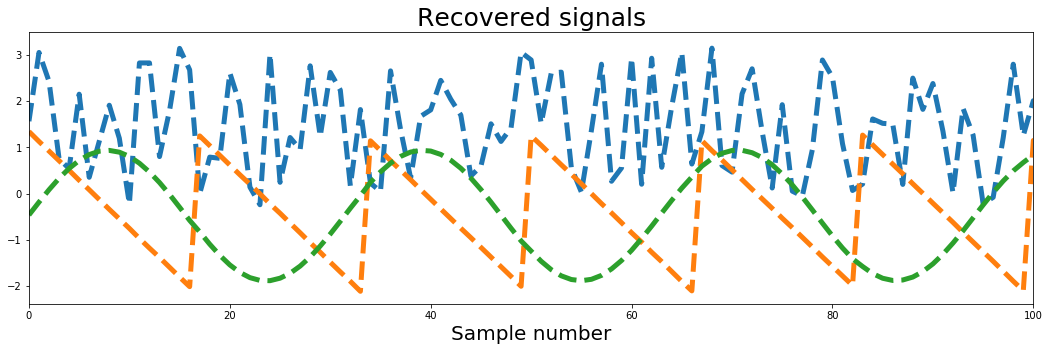
fig, ax = plt.subplots(1, 1, figsize=[18, 5])
ax.plot(S, lw=5)
ax.tick_params(labelsize=12)
ax.set_xticks([])
ax.set_yticks([-1, 1])
ax.set_title('Source signals', fontsize=25)
ax.set_xlim(0, 100)
fig, ax = plt.subplots(1, 1, figsize=[18, 5])
ax.plot(unMixed, '--', label='Recovered signals', lw=5)
ax.set_xlabel('Sample number', fontsize=20)
ax.set_title('Recovered signals', fontsize=25)
ax.set_xlim(0, 100)
plt.show()
FastICA and maximum likelihood
$$w^{+} = w - \frac{1}{E[g^{'}(w^Tx)] - \beta}[E[xg(w^T x)] - \beta w]$$
=> The Fixed-Point Algorithm and Maximum Likelihood Estimation for Independent Component Analysis (1999)
$$w^{+} = w + D[diag(-\beta_i)+E[g(y)y^T]]W$$
$$(D = diag(1/(\beta_i - E[g^{'}(y_i)])))$$
$$w^{+} = w + u[I+g(y)y^T]w$$
u를 Learning Rate로서 설정하여서 점차적으로 접근하는 방식을 사용할 수 있다.
아직 논문을 보는 중이면 이해하지 못하였습니다.
Parallel ICA
FMRI: $y_1 = w_1*s_1$
SNPS: $y_2 = w_2*s_2$
2개 Weight Update -> $w_1, w_2$의 Correlation이 높게 W update
Matlab 사용: Matlab Tool
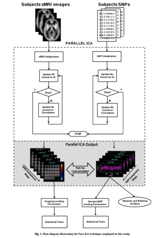
Advantages of Parallel ICA
Data의 형태가 다음과 같다고 생각해보자.
$$FMRI = [voxel_1, voxel_2, ....]$$
$$SNP = [snp_1, snp_2, ....]$$
위와 같은 Data로서는 univariate Analysis를 주로 사용할 것이다. 즉, 어떤 SNP의 구성요소와 어떤 FMRI의 구성요소가 상관있는지 나타낼 것이다.
하지만 Parallel ICA를 사용하게 되면 Large Scale에서 Multivariate Analysis가 가능하다.
우리는 Parallel ICA를 통해서 다음과 같은 Independent한 Source를 얻었다고 하자.
$$Source FMRI = [svoxel_1, svoxel_2, ...]$$
$$Source SNP = [ssnp_1, ssnp_2, ...]$$
만약 $svoxel_1$과 $ssnp_1$이 높은 Correlation관계를 보인다면 이는 다음과 같이 나타낼 수 있다.
$$svoxel_1 = \alpha_1*voxel_1 + \alpha_2*voxel_2, ...$$
$$ssnp_1 = \beta_1*snp_1 + \beta_2*snp_2, ...$$
위에서 각각의 $\alpha, \beta$에 z score가 큰 특정 $\alpha, \beta$만 남긴다고 생각하면 다음과 같이 나타낼 수 있다.
$$svoxel_1 = \alpha_1*voxel_1 + \alpha_2*voxel_2$$
$$ssnp_1 = \beta_1*snp_1 + \beta_2*snp_2$$
=>SNP의 특정 몇개의 조합과 FMRI에서 특정 Voxel의 조합이 상관 있다 라는 것을 확인할 수 있다.
참고
각각의 Data를 독립적으로 ICA로 분리하고 Correlation으로서 분석하는 것 보다 Parallel ICA로서 Correlation을 분석하는 것이 더 결과가 좋았다는 다른 논문(COmbining fMRI and SNP Data to Investigate Connections Between Brain Function and Genetics Using Parallel ICA)에 주장이 있습니다.
Leave a comment