
Theory12. Matrix Factorization
Multi-Modality Disease Modeling via Collective Deep Matrix Factorization
(https://dl.acm.org/doi/pdf/10.1145/3097983.3098164)
Abstract
The challenging task of MCI detection is therefore of great clinical importance. We propose a framework to fuse multiple data modalities for predictive modeling using deep matrix factorization, which explores the non-linear interactions among the modalities and exploits such interactions to transfer knowledge and enable high performance prediction.
주요한 점은 2가지 이다. 현재 NL -> MCI -> AD로 가기전에 MCI를 발견하는 것이 큰 목표이며, 이러한 MCI발견을 위하여 여러가지 Modality를 Funsion하여 MCI를 Prediction을 하겠다는 것 이다.
여러 가지 Modality를 Fusion하기 위하여 Collective Matrix Factorization에서 Non-Linearlity를 증가시키기 위하여 Collective Deep Matrix Factorization을 사용하였다.
Matrix Completetion
Matrix Factorization기법은 Recommend System에서 많이 사용하는 방법 중 하나이다.
먼저 Recommend System에서의 사용방법을 사용하기 위하여 다음과 같은 예제를 생각해보자.
사진 출처: sanghyukchun 블로그
위와같이 특정 User에게 Movie를 추천하려고 하나 모든 정보가 없기 때문에 추천할 수 없는 상황이 있다.
이러한 비어있는 Matrix를 채우기 위하여 Matrix Factorization을 사용하게 된다.
이러한 Matrix를 채우는 문제를 Matrix Completion이라고 칭하게 된다.
Matrix Factorization
Matrix Completion을 위하여 사용하는 방법이다.
Matrix Factorization의 수식은 매우 간단하다.
$$\hat{r_{ui}} = p_u \cdot q_i$$
$$min\text{ }rank(\hat{R}) \text{ s.t. }\Omega(r_{ui}-\hat{r_ui}) = 0 \forall u,i$$
$$ \Omega(A_{ij}-B_{ij})= \begin{cases} 0, & \mbox{if }A_{ij} \mbox{or }B_{ij} = 0 \\ A_{ij}-B{ij}, & \mbox{else} \end{cases} $$
위의 수식을 살펴보게 되면 매우 간단하다는 것을 알 수 있다.
실제 가지고 있는 Matrix를 \(r_{ui}\)라고 가정하면 이 Matrix를 \(p_u, q_i\)로서 나누게 된다.
즉, \(r_{ui} \in R^{n*m}\)이라면, \(p_u \in R^{n*r}, q_i \in R^{m*r}\), \(r << n,m\)이라고 생각하자.
다시 생각해보면, Original Matrix의 Rank는 줄일수 있으며, 이로 인하여 Low Rank Matrix로서 나눌 수 있다. 이러한 Rank를 줄일 수록, Dimension Reduction은 더 가능할 것 이다.
예제로서 생각해보면, 아래와 같을 것 이다.
user u의 item들에 대한 숨겨진(latent) interest \(p_u\)와 그에 대응하는 item들의 숨겨진 특성 \(q_i\)에 의해 결정된다는 사실을 알 수 있다. 이를 그림으로 표현하면 다음과 같다.
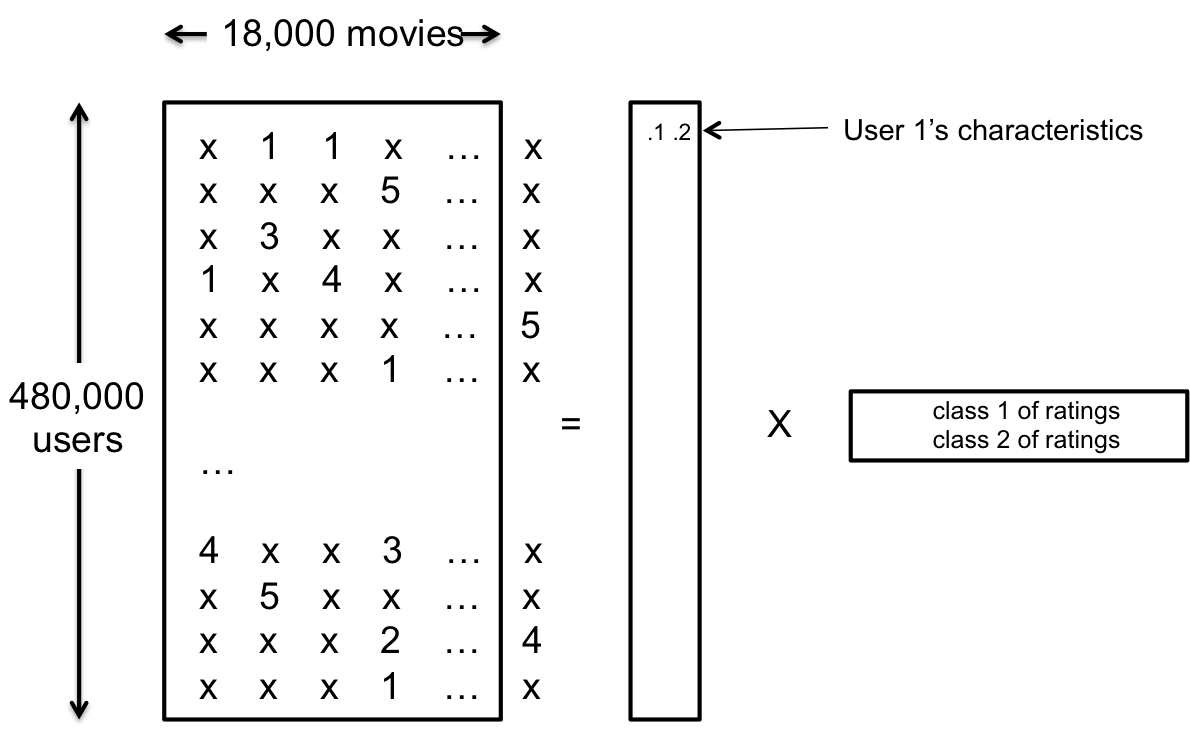
사진 출처: sanghyukchun 블로그
Matrix Factorization Solution
다시한번 Matrix Factorization의 식을 살펴보면 다음과 같다.
$$min\text{ }rank(\hat{R}) \text{ s.t. }\Omega(r_{ui}-\hat{r_ui}) = 0 \forall u,i$$
위와 같이 Rank자체를 Minimize하는 Rank Condition은 Non-Convex 문제 이므로 Optimization을 할 수 없다. 따라서 위와 같은 형태를 Convex한 문제로서 변형하는 것은 다음과 같이 2가지 방법이 있다.
1. Convex Relaxation
위의 수식의 Rank를 최소화 하는 문제는 다음과 같이 생각할 수 있다.
$$min \sum_{l}||\sigma_{l}(\hat{R})||_{0} \text{ s.t.} \Omega(r_{ui}-\hat{r_{ui}})=0 \forall u,i$$
Singular value를 구하고 이가 0이 아닌 값을 Count하는 l0 Norm으로서 나타낼 수 있다는 것 이다.
Singular Value를 Count하는 문제는 위에서 언급한 대로 Non-Convex한 문제이기 때문에 다음과 같이 식을 변형한다.
$$norm||R||_{*}$$
l0 norm -> l1 or l2 …. norm으로서 변형하면서 Convex한 형태로 만드는 것을 Convex Relaxation이라고 칭한다.
이러한 방식은 GLobal한 Optimal값을 찾을 수 있지만, 결국 Data에 너무 의존하는 형태가 될 것이다.
2. Solve Non-Convex Problem Directly
$$min_{\hat{R}} \sum_{u,i \in k}(r_{ui} - \hat{r_{ui}}) \text{ s.t }rank(\hat{R} = k)$$
위의 수식을 살펴보게 되면 원래 Matrix Factorization의 Minimize시겡서 s.t.와 Formulation이 변형된 것을 알 수 있다.
Rank(줄이고자 하는 Dimension)은 고정시키고, 이 Rank에서 s.t를 만족하는 것으로서 Solution을 찾겠다는 의미이다. Global한 Solution값을 찾을 수 없겠지만, Grid Search방식으로서 Local Minimum은 찾을 수 있을 것이고, 이러한 형태는 꽤 성능이 좋다고 알려져 있다.
위와 같은 Matrix Factorization은 Overfitting을 피하기 위하여 다음과 같은 방식으로 Trainning된다.
$$min_{P,Q} \sum_{u,i \in k}(r_{ui} - p_{u}\cdot q_i)^2 + \lambda(||p_u||_{2}^2+||q_i||_{2}^2)$$
Collective Matrix Factorization
위와 같은 Matrix Factorization은 Univariate Analysis인 것을 확인할 수 있을 것 이다.(위에서는 User-Movie로서 1:1 Mapping)
Multimodality Analysis를 위하여 Collective Matrix Factorization을 사용하게 된다.
실제 Paper에서의 수식을 살펴보게 되면 다음과 같다.
$$min_{U,V_1,V_2} d(X_1,UV_1^T)+d(X_2,UV_2^T) \text{ s.t} U \in S_0, V_i \in S_{i}, i=1,2$$
Matrix Factorization처럼 예시로서 설명하면 다음과 같다.
우리는 n명에 대한 Sample이 있고, 각각 SMRI, SNPs의 Data를 가지고 있다고 생각하면 각각의 Data를 다음과 같이 나타낼 수 있다.
- \(X_1 \in R^{r*d_1}\): MRI Data
- \(X_2 \in R^{r*d_2}\): SNPs Data
Sample의 수는 같을 것이고 Data의 특성에 따라서 Dimension이 달라지게 될 것이다.
이러한 Data를 Matrix Factorization으로서 나누게 되면 다음과 같이 나눠질 수 있다.
- \(X_1 = UV_1 \text{ s.t }U \in R^{n*r}, V_1 \in R^{r*d_1}\)
- \(X_2 = UV_2 \text{ s.t }U \in R^{n*r}, V_2 \in R^{r*d_2}\)
즉, 각각의 Matrix Factorization에서의 각각의 Sample에 대한 특성은 공유하면서, Data에 따라서 특성이 다르게 Matrix Factorization이 가능하다는 것 이다.
공통적인 특성인 U를 공유함으로서 Multi Modality Analysis가 가능하다는 것 이다.
Collective Deep Matrix Factorization

위의 Figure는 현재 Paper에서 설명하는 Collective Deep Matrix Factorization에 대한 내용이다.
Collective Matrix Factorization에서 Non-Linearity를 증가시키기 위하여 ANN을 사용했다는 것 이다.
수식으로서 살펴보면 다음과 같다.
$$min_{U, (V_i, \theta_i)_{i=1}^{t}} \sum_{i=1}^{t} d(X_i,U g_{\theta_i}(V_i)) \text{ s.t} U \in S_0, V_i \in S_i$$
$$g_{\theta_i}(V_i) = f(W_{(k,i)}f(W_{(k-1,i)}f(...,W_{(1,i)}V_i))$$
위의 식을 Collective Matrix Factorization과 비교하면 \(V \rightarrow g_{\theta_i}(V_i)\)로서 ANN의 결과로서 사용하는 것을 살펴볼 수 있다.
즉, Collective Deep Matrix Factorization의 핵심은 다음과 같다.
- U를 공유함으로서 Multi-Modality Analysis가 가능하다.
- U를 통하여 Prediction하는 경우에 Dimension Reduction이 된다.
- ANN을 사용하여 단순한 Matrix Multiply가 아닌 Matrix * ANN으로서 Non-Linearity를 증가시켰다
실제 Trainning과 각각의 Modality의 Significant를 측정하기 위하여 최종적인 식은 다음과 같이 정의하였다.
$$min_{U, (V_i, \theta_i)_{i=1}^{t}} \sum_{j=1}^{n} l(h(U_j;w),y_j) + \sum_{i=1}^{t} \alpha_i d(X_i,U g_{\theta_i}(V_i)) \text{ s.t} U \in S_0, V_i \in S_i, \forall_i$$
$$l(h(U_j;w),y_j): \text{ Logistic Regression}$$
$$g_{\theta_i}: \text{ Same architecture and share the same parameter values, except for the last layer}$$
최종적인 목적은 Dataset에 대하여 NL or MCI로서 판단하는 것 이다.
식을 살펴보게 되면 크게 2개의 Term으로서 이루워질 수 있는 것을 볼 수 있고 각각은 다음과 같은 의미를 가지고 있다.
- 1 Term: \(l(h(U_j;w),y_j)\): U(Latent Representation)으로서 NL or MCI를 Prediction
- 2 Term: \(\alpha_i d(X_i,U g_{\theta_i}(V_i))\): U를 Update하기 위하여 사용한다. \(\alpha_i\)를 통하여 각각의 Modlaity의 중요도를 결정하게 된다. 만약 \(\alpha_i\)가 크다면, 그 Modality에 대하여 같은 Epoch에 대하여 더 Trainning을 잘 보게 될 것이다. 즉, \(\alpha_i\)가 클수록 Modality에 대한 중요도를 높인 것이라고 생각할 수 있다.
Appendix
Initialization
현재 논문에서는 다음과 같이 표현하고 있다.
Since the objective in highly non-convex and gradient algorithms may easily trapped in local optima, a good initialization is important for training the network => Initialization: SVD
위에서 적은 Matrix Factorization의 문제를 살펴보게 되면, 다음과 같은 문제가 있는 것을 확인할 수 있었다.
- Matrix Factorization의 Cost Funciton은 Non-Convex이므로 Optimal한 값을 찾을 수 없다.
- Convex Relaxation으로서 Optimal Solution을 찾을 수 있지만, Data에 너무 의존하게 되어서, 식이 성립안할 수 있다.
- 위와 같은 문제로 인하여 Non-convex Problem으로서 Directly로 구하게 되면, Rank자체를 고정하고, 그에 따른 Local Optimum을 찾는 문제로서 해결한다.
이러한 Local Optimum에 빠지게 되는 것을 최대한 방지하고자 하는 방법이 Initialization으로서 SVD를 사용하는 것이다.
현재 Paper에서도 Initialization을 SVD를 사용하여 성능을 향상시켰다고 한다.
Initialization을 SVD로서 사용하는 이유는 논문을 참조하자
논문: SVD based initialization: A head start for nonnegative matrix factorization
(https://www.sciencedirect.com/science/article/pii/S0031320307004359)
Imaging modalities preprocessing
현재 논문에서는 ADNI1, ADNI2에 대하여 사용하였다.
또한 논문에서 강조하고 있는 것이 Image를 Preprocessing하는 과정에서 Age와 Sex, 그리고 각각의 Data 특성을 고려해야 한다는 것 이다.
해당 Formulation은 다음과 같다.
$$X^{obs} = w_1 \cdot age + w_2 \cdot sex + w_3 \cdot cohort + X^{ori}$$
- \(X^{obs}\): 실제 값
- \(X^{ori}\): age, sex, cohort와 관계가 없는 값(사용하고자 하는 값)
- \(cohort\): ADNI1: 1, ADNI2: -1
실제Training은 다음과 같이 진행된다.
$$w^{*} = min_w \sum_{i=1}^{n} (x^t t_i-X_i^{obs})^2$$
따라서 위와 같이 실제 Data인 \(X^{obs}\)에 대하여 age, sex, cohort로서 표현 가능하면 이러한 영향이 없는 \(X^{ori}\)는 다음과 같이 적을 수 있다.
$$X^{ori} = X^{obs} - (w_1^{*}\cdot age+w_2^{*}\cdot sex+w_3^{*}\cdot cohort)$$
Age correction등이 MRI Image을 통하여 Classification에서 성능이 향상된 예시는 해당 논문은 다음과 같다.
논문: The Effect of Age Correction on Multivariate Classification in Alzheimer’s Disease, with a Focus on the Characteristics of Incorrectly and Correctly Classified Subjects
(https://www.ncbi.nlm.nih.gov/pmc/articles/PMC4754326/)
위의 논문에서 Age Correction Method부분을 살펴보면 다음과 같이 이야기 하고 있다.
The detrending algorithm fits a generalized linear model (GLM) to each MRI-derived variable and age, in the CTL group only, and models the age-related changes as a linear drift. Then, the regression coefficient of the resulted GLM model (linear drift) is used to remove the age-related changes from all individuals (AD, MCI and CTL) and obtain corrected values. The linear model was chosen based on the Good et al. (2001) study where they found an age-related linear decrease in global grey matter volume in healthy individuals.
GrayMatter는 Age가 많아짐에 따라서 Linear Decrease가 있기 때문에, 이에 따른 Correction을 하여 Dataset에서 Age에 대한 Effect가 없어지도록 Preprocessing하는 것이 Model의 성능을 향상시킨다는 것 이다.
Result
Result의 경우에는 크게 2가지로 나누어서 생각할 수 있다.
1. Predict Performance
실제 MRI or NL을 Prediction하는 Model의 성능에 대하여 해당 논문은 다음과 같은 Performance를 보여주었다고 한다.
Prediction performance of different models using ADNI2’s T1 MRI and dMRI in terms of AUC. With an appropriate activation function and components’ number, our method outperfoms than all other methods.
Prediction performance of different models using ADNI2’s and ADNI1’s T1 MRI and dMRI in terms of AUC. With an appropriate activation function and components’ number, our method outperfoms than all other methods.
Prediction performance of fusing genetic knowledge and imaging knowledge using ADNI1 and ADNI2 in terms of AUC. Genetic modality can be successfully integrated with imaging modalities.
Components란 \(g_{\theta_i}(V_i)\)의 2번째 Layer를 의미하게 되고, 각각의 Activation Function과 Model을 바꿔가면서 측정한 결과이다.
중요하게 봤던 점은 Genetic Data를 추가함으로서 AUC가 증가한다는 것 이다. 즉, Image Data와 Genetic Data를 활용하여 Multivariate Analysis를 휼륭하게 수행하였다는 점 이다.
2. Effects of knowledge fusion parameters
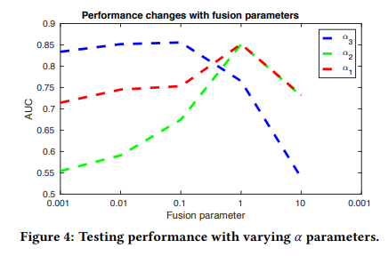
- \(\alpha_1\): dMRI
- \(\alpha_2\): T1
- \(\alpha_3\): SNPs
위의 LossFunction을 다시 살펴보면 다음과 같다.
$$min_{U, (V_i, \theta_i)_{i=1}^{t}} \sum_{j=1}^{n} l(h(U_j;w),y_j) + \sum_{i=1}^{t} \alpha_i d(X_i,U g_{\theta_i}(V_i)) \text{ s.t} U \in S_0, V_i \in S_i, \forall_i$$
위의 식에서 \(\alpha_i\)를 변형시켜가면서 얻은 Model의 AUC에 대한 Graph이다.
\(\alpha_1, \alpha_2\)는 같은 Image Data로서 값이 비슷하게 변하는 결과를 보여주었다면, \(\alpha_3\)의 경우는 0.1을 넘는순간 급격하게 AUC가 감소되는 것을 확인할 수 있다.
이러한 결과에 대하여 해당 Paper는 다음과 같이 얘기하고 있다.
That is because genetic modality is noiser than imaging modalityies. With a small a3, , this model can tolerant a lager reconstruction error for genetic modality. Hence, the model is robust to the noise in genetic modality.
Genetic Data가 Image Data보다 Noise가 많다는 것 이고, 이에 따라서 \(\alpha_3\)의 값을 작게하여서, Noise에 대하여 Robust한 Model을 구축하였다고 한다.
Collective Deep Matrix Factorization 구현
1
2
3
4
5
6
7
8
9
10
11
12
import pandas as pd
import torch
import numpy as np
import os
import torch.nn as nn
import torch.optim as optim
import torch.nn.init as init
import matplotlib.pyplot as plt
import math
from sklearn.metrics import roc_auc_score
import torch.nn.functional as F
import matplotlib.pyplot as plt
LossFunction
$$min_{U, (V_i, \theta_i)_{i=1}^{t}} \sum_{j=1}^{n} l(h(U_j;w),y_j) + \sum_{i=1}^{t} \alpha_i d(X_i,U g_{\theta_i}(V_i)) \text{ s.t} U \in S_0, V_i \in S_i, \forall_i$$
$$l(h(U_j;w),y_j): \text{ Logistic Classification - NL_MCI or NL_AD}$$
$$l(h(U_j;w),y_j): \text{ Softmax Classification - NL_MCI_AD}$$
$$g_{\theta_i}: \text{ Same architecture and share the same parameter values, except for the last layer}$$
- Term1 Loss: It can be seen that it is a typical Loss of CLassification Model
- NL_MCI or NL_AD: Logistic Regression Model(Sigmoid)
-
NL_MCI_AD: SoftMax => Label is One-Hot-Encoding
- Term2 Loss: It can be seen that L2 Loss was used as the loss of the problem of restoring the original data
Reference
Overfitting occurs due to the small number of samples.
Therefore, L2 Regularization, one of the mothods to avoid overfitting, is used as the Term2 Loss declared.
1
2
3
4
5
6
7
8
9
10
11
12
13
14
15
16
def sigmoid(x):
    return 1/(1+torch.exp(-x))

# Term2 Loss & Regularization
def frob(z):
    vec_i = torch.reshape(z,[-1])
    return torch.sum(torch.mul(vec_i,vec_i))

# Term1 Loss
# 1 Dimension Loss
def logistic_loss(label,y):
    return -torch.mean(label*torch.log(y)+(1-label)*(torch.log(1-y)))

# One-Hot Loss
def logistic_loss2(label,y):
    return -torch.mean(torch.sum(label*torch.log(y),axis=1))
Utility
Data Load
1
2
3
4
5
6
7
8
9
10
11
12
13
14
15
16
17
18
19
20
21
22
def load_data(file_path,NL_MCI_AD=False):
    if NL_MCI_AD:
        X_roi = pd.read_csv(file_path+'X_roi.csv', index_col=0)
        X_roi = torch.tensor(X_roi.values,dtype=torch.double,requires_grad=False)

        X_snp = pd.read_csv(file_path+'X_snp.csv', index_col=0)
        X_snp = torch.tensor(X_snp.values,dtype=torch.double,requires_grad=False)

        Y = np.load(file_path+'Label.npy')
        Y_Label = torch.tensor(Y,dtype=torch.double, requires_grad=False)

    else:
        X_roi = pd.read_csv(file_path+'X_roi.csv',index_col=0)
        X_roi = torch.tensor(X_roi.values,dtype=torch.double,requires_grad=False)

        X_snp = np.load(file_path+'X_snp.npy')
        X_snp = torch.tensor(X_snp,dtype=torch.double,requires_grad=False)

        Y_Label = pd.read_csv(file_path+'Label.csv',index_col=0)
        Y_Label = torch.tensor(Y_Label.values,dtype=torch.double,requires_grad=False)

    return X_roi,X_snp,Y_Label
SVD Initialization
This is one of the ways to improve the performance of Matrix Factorization.
The output of SVD is finally expressed as \(U\sum V^{T}\) and the value of SVD is sorted and displayed through np.linalg.svd.
In other words, it can be expressed as a Diemnsion Reduction Matrix expressed as a matrix with a large EigenValue according to the dimension to be used.
When referring to Paper (Collective Deep Matrix Factorization), you can see how many Eigenvalues of each SVD should be used as Hyperparameters and use the best performance.
1
2
3
4
5
6
7
8
9
10
11
12
13
14
15
16
17
18
19
20
21
22
23
24
25
26
27
28
29
30
31
32
33
34
35
36
37
38
39
40
41
42
43
44
45
46
47
def svd_initialization(X_roi, X_snp, du1, du2, NL_MCI_AD=False):
    train_size = int(X_roi.shape[0]*0.9)

    u_roi_svd1, _, v_roi_svd1 = np.linalg.svd(X_roi,full_matrices=False)
    u_roi_svd2, _, v_roi_svd2 = np.linalg.svd(u_roi_svd1,full_matrices=False)

    # SNP => One-Hot-Encoding
    if NL_MCI_AD:
        u_snp_svd1, _, v_snp_svd1 = np.linalg.svd(X_snp,full_matrices=False)
        u_snp_svd2, _, v_snp_svd2 = np.linalg.svd(u_snp_svd1,full_matrices=False)


        v_snp = torch.tensor(v_snp_svd1[0:du1, :], dtype=torch.double, requires_grad=True)
        u_snp = torch.tensor(u_snp_svd2[0:du2,0:du1], dtype=torch.double, requires_grad=True)

        w = torch.empty(du2, 3,dtype=torch.double,requires_grad=True)
        b = torch.zeros(1,3,dtype=torch.double, requires_grad=True)

    # SNP => Category Value: 0 or 1 or 2
    else:
        v_snp = np.zeros((du1,X_snp.shape[1],3))
        u_snp = np.zeros((du2,du1,3))

        for i in range(3):
            u_snp_svd1, _, v_snp_svd1 = np.linalg.svd(X_snp[:,:,i],full_matrices=False)
            u_snp_svd2, _, v_snp_svd2 = np.linalg.svd(u_snp_svd1,full_matrices=False)

            v_snp[:,:,i] = v_snp_svd1[0:du1, :]
            u_snp[:,:,i] = u_snp_svd2[0:du2,0:du1]

        v_snp = torch.tensor(v_snp,dtype=torch.double, requires_grad=True)
        u_snp = torch.tensor(u_snp,dtype=torch.double, requires_grad=True)

        w = torch.empty(du2, 1,dtype=torch.double,requires_grad=True)
        b = torch.zeros(1,dtype=torch.double, requires_grad=True)

    v_roi = torch.tensor(v_roi_svd1[0:du1, :],dtype=torch.double, requires_grad=True)
    u_roi = torch.tensor(u_roi_svd2[0:du2,0:du1],dtype=torch.double, requires_grad=True)

    u = torch.tensor(u_roi_svd2[:,0:du2],dtype=torch.double, requires_grad=True)

    # Xavier Initialization
    nn.init.xavier_uniform_(w)

    b = torch.tensor(0.1,dtype=torch.double,requires_grad=True)

    return u,u_roi,v_roi,u_snp,v_snp,w,b
Train
There are two models.
Model that distinguishes NL_MCI or NL_MCI_AD (Model1)
Model that distinguish NL_MCI_AD (Model2)
Model 1
In the case of Model 1, the output is composed of Sigmoid because the Label is a Category Value (0 or 1). In addition, One-Hot-Encoding was used to classify SNPs Data having the same category value as Paper (Collective Deep Matrix Factorization).
- SNPs Data
- 0: [1,0,0]
- 1: [0,1,0]
- 2: [0,0,1]
Model 2
In the case of Model2, Label is indicated as One-Hot-Encoidng.
- Label
- NL: [1,0,0]
- MCI: [0,1,0]
- AD: [0,0,1]
Unlike Model 1, SNPs Data is not shown as One-Hot-Encoding.
This is because overfitting occurs because the number of weights to be trained becomes too large when expressed as one-hot encoding to SNPs data. Therefore, the value of 0 or 1 or 2 was used as it is.
1
2
3
4
5
6
7
8
9
10
11
12
13
14
15
16
17
18
19
20
21
22
23
24
25
26
27
28
29
30
31
32
33
34
35
36
37
38
39
40
41
42
43
44
45
46
47
48
49
50
51
52
53
54
55
56
57
58
59
60
61
62
63
64
65
66
67
68
69
70
71
72
73
74
75
76
77
78
79
80
81
82
83
84
85
86
87
88
89
90
91
92
93
94
95
96
97
98
99
100
101
102
103
104
105
106
107
108
109
def train(max_steps, tol, file_path, du1, du2, alpha1=1, alpha2=1, NL_MCI_AD=False):
    # Data Load
    X_roi,X_snp,Y_Label = load_data(file_path,NL_MCI_AD)

    # Train Test split parameter => 0.9:1
    train_size = int(X_roi.shape[0]*0.9)
    sample_size = X_roi.shape[0]

    # SVD Initialization
    u,u_roi,v_roi,u_snp,v_snp,w,b = svd_initialization(X_roi,X_snp,du1,du2, NL_MCI_AD)

    # Label Split
    y_ = Y_Label[0:train_size,:]
    y__ = Y_Label[train_size:sample_size,:]

    # Optimizer
    optimizer = torch.optim.Adam([u,u_roi,v_roi,u_snp,v_snp,w,b], lr=1e-4)

    # For Model Performance
    funval = [0]

    for i in range(max_steps+1):
        # Overfitting => 1. Dropout
        u_train = u[0:train_size,:]
        u_train = torch.dropout(u_train,p=0.3,train=True)

        if NL_MCI_AD:
            roi_ = torch.matmul(u,torch.sigmoid(torch.matmul(u_roi,v_roi)))
            snp_ = torch.matmul(u,torch.sigmoid(torch.matmul(u_snp,v_snp)))
            prediction_ = F.softmax(torch.matmul(u_train,w)+b, dim=1)

            # Model Loss
            prediction_loss = logistic_loss2(y_,prediction_)+alpha1*frob(X_roi-roi_)+alpha2*frob(X_snp-snp_)

        else:
            roi_ = torch.sigmoid(torch.matmul(u,torch.square(torch.matmul(u_roi,v_roi))))

            # Becuas of One-Hot-Encoding
            snp_0 = torch.sigmoid(torch.matmul(u,torch.square(torch.matmul(u_snp[:,:,0],v_snp[:,:,0]))))
            snp_1 = torch.sigmoid(torch.matmul(u,torch.square(torch.matmul(u_snp[:,:,1],v_snp[:,:,1]))))
            snp_2 = torch.sigmoid(torch.matmul(u,torch.square(torch.matmul(u_snp[:,:,2],v_snp[:,:,2]))))
            snp_ = torch.stack([snp_0,snp_1,snp_2],axis=2)

            prediction_ = torch.sigmoid(torch.matmul(u_train,w)+b)

            # Model Loss
            prediction_loss = logistic_loss(y_,prediction_)+alpha1*frob(X_roi-roi_)+alpha2*frob(X_snp-snp_)

        # Overfitting => 2. L2 Regularization
        regularization_loss = 0.01*frob(u_roi) + 0.01*frob(u_snp)+ 0.01*frob(u) + 0.01*frob(v_roi) + 0.01*frob(v_snp)

        # Total Loss
        total_loss = prediction_loss+regularization_loss

        # Weight Update
        optimizer.zero_grad()
        total_loss.backward(retain_graph=True)
        optimizer.step()

        # When there is no improvement in model performance
        total_loss_digit = total_loss.detach().item()
        funval.append(total_loss_digit)

        if abs(funval[i+1]-funval[i]) < tol:
            train_auc = roc_auc_score(y_.detach(),prediction_.detach())
            print('Early Stopping')
            train_auc = roc_auc_score(y_.detach(),prediction_.detach())
            print('Iteration: ',i,' Train_AUC:',train_auc)

            if NL_MCI_AD:
                print("Label: ",y_.detach()[25:30])
                print("Model Prediction: ", prediction_.detach()[25:30],'\n')

            else:
                print("Label: ",y_.detach()[10:15].T)
                print("Model Prediction: ", prediction_.detach()[10:15].T,'\n')
            break

        # Wrong Model Loss
        if math.isnan(total_loss):
            print("Totla Loss Exception2")
            print(funval)
            break

        # Metric: AUC Score
        # 1. Train AUC
        if i%5000 == 0:
            train_auc = roc_auc_score(y_.detach(),prediction_.detach())
            print('Iteration: ',i,' Train_AUC:',train_auc)

            if NL_MCI_AD:
                print("Label: ",y_.detach()[25:30])
                print("Model Prediction: ", prediction_.detach()[25:30],'\n')

            else:
                print("Label: ",y_.detach()[10:15].T)
                print("Model Prediction: ", prediction_.detach()[10:15].T,'\n')

    # 2. Test AUC
    u_test = u.detach()[train_size:sample_size,:]

    if NL_MCI_AD:
        prediction__ = F.softmax(torch.matmul(u_test,w)+b, dim=1)
    else:
        prediction__ = torch.sigmoid(torch.matmul(u_test,w)+b)

    test_auc = roc_auc_score(y__.detach(),prediction__.detach())

    return train_auc,test_auc
Component Select
CDMF (Collective Deep Matrix Factorization) is an EM algorithm.
- Model performance may vary depending on the number of components.
- Model performance may vary depending on the weight initialization.
In the case of 2, we could not find the Global Optimum in SVD Initialization, but we could confirm that it finds a good performance in Local Minimum.
In the case of 1, there are many methods, but the number of components was determined while changing the Hyperparameter of the Model.
1
2
3
4
5
6
7
8
9
10
11
12
13
14
15
16
17
18
19
20
21
22
23
24
25
26
27
28
29
30
31
32
33
34
35
36
37
38
39
40
41
42
43
44
45
46
47
48
49
50
51
52
# File Path
subject = ['NL_MCI','NL_AD','NL_MCI_AD']
file_path = ['./data/'+subject[0]+'_Data/', './data/'+subject[1]+'_Data/', './data/'+subject[2]+'_Data/']

# Hyperparameter
max_iter = 20000
tol = 1e-7
du1 = [50,100,150]
du2 = [30,50,70,90,110,130]

# Result List
nl_mci_list = []
nl_ad_list = []
nl_mci_ad_list = []

print('Component Select\n')

for i,f in enumerate(file_path):
    # Component Select Result Write
    directory = f+'Component_Select_Result'
    if not os.path.exists(directory):
        os.makedirs(directory)

    aucfile = open(directory+'/auc2.txt','a')


    # du1: Component 1, du2: Component 2
    for d1 in du1:
        for d2 in du2:
            print(subject[i]+' Trainning '+"Component1: "+str(d1)+" Component2: "+str(d2))

            # NL_MCI
            if i == 0:
                train_auc,test_auc = train(max_iter,tol,f,d1,d2)
                nl_mci_list.append(test_auc)

            # NL_AD
            elif i == 1:
                train_auc,test_auc = train(max_iter,tol,f,d1,d2)
                nl_ad_list.append(test_auc)

            # NL_MCI_AD
            else:
                train_auc,test_auc = train(max_iter,tol,f,d1,d2,NL_MCI_AD=True)
                nl_mci_ad_list.append(test_auc)

            # Write Result
            aucfile.write("Component1: %s Component2: %s Train_AUC: %s Test_AUC: %s\n"%(str(d1),str(d2),str(train_auc),str(test_auc)))

            print('Model Test: ',test_auc,'\n\n')

    aucfile.close()
1
2
3
4
5
6
7
8
9
10
11
12
13
14
15
16
17
18
19
20
21
22
23
24
25
26
27
28
29
30
31
32
33
34
35
36
37
38
39
40
41
42
43
44
45
46
47
48
49
50
51
52
53
54
55
56
57
58
59
60
61
62
63
64
65
66
67
68
69
70
71
72
73
74
75
76
77
78
79
80
81
82
83
84
85
86
87
88
89
90
91
92
93
94
95
96
97
98
99
100
101
102
103
104
105
106
107
108
109
110
111
112
113
114
115
116
117
118
119
120
121
122
123
124
125
126
127
128
129
130
131
132
133
134
135
136
137
138
139
140
141
142
143
144
145
146
147
148
149
150
151
152
153
154
155
156
157
158
159
160
161
162
163
164
165
166
167
168
169
170
171
172
173
174
175
176
177
178
179
180
181
182
183
184
185
186
187
188
189
190
191
192
193
194
195
196
197
198
199
200
201
202
203
204
205
206
207
208
209
210
211
212
213
214
215
216
217
218
219
220
221
222
223
224
225
226
227
228
229
230
231
232
233
Component Select

NL_MCI Trainning Component1: 50 Component2: 30
Iteration:  0  Train_AUC: 0.5259622713414634
Label:  tensor([[1., 1., 1., 0., 1.]], dtype=torch.float64)
Model Prediction:  tensor([[0.5037, 0.5053, 0.5317, 0.5256, 0.5092]], dtype=torch.float64)

Iteration:  5000  Train_AUC: 0.8408123729674797
Label:  tensor([[1., 1., 1., 0., 1.]], dtype=torch.float64)
Model Prediction:  tensor([[0.6437, 0.7286, 0.6833, 0.5302, 0.7210]], dtype=torch.float64)

Iteration:  10000  Train_AUC: 0.8605500508130081
Label:  tensor([[1., 1., 1., 0., 1.]], dtype=torch.float64)
Model Prediction:  tensor([[0.7048, 0.9373, 0.9004, 0.6101, 0.9531]], dtype=torch.float64)

Iteration:  15000  Train_AUC: 0.8662665142276423
Label:  tensor([[1., 1., 1., 0., 1.]], dtype=torch.float64)
Model Prediction:  tensor([[0.8856, 0.9109, 0.8930, 0.6443, 0.9800]], dtype=torch.float64)

Iteration:  20000  Train_AUC: 0.883812881097561
Label:  tensor([[1., 1., 1., 0., 1.]], dtype=torch.float64)
Model Prediction:  tensor([[0.8709, 0.7317, 0.8731, 0.6046, 0.9977]], dtype=torch.float64)

Model Test:  0.8661518661518661


...


NL_MCI Trainning Component1: 150 Component2: 130
Iteration:  0  Train_AUC: 0.4726880081300813
Label:  tensor([[1., 1., 1., 0., 1.]], dtype=torch.float64)
Model Prediction:  tensor([[0.5137, 0.5152, 0.5211, 0.5138, 0.5286]], dtype=torch.float64)

Iteration:  5000  Train_AUC: 0.9051861026422764
Label:  tensor([[1., 1., 1., 0., 1.]], dtype=torch.float64)
Model Prediction:  tensor([[0.7245, 0.7534, 0.6779, 0.4535, 0.9177]], dtype=torch.float64)

Iteration:  10000  Train_AUC: 0.9360391260162602
Label:  tensor([[1., 1., 1., 0., 1.]], dtype=torch.float64)
Model Prediction:  tensor([[0.9282, 0.9567, 0.4559, 0.3447, 0.9489]], dtype=torch.float64)

Iteration:  15000  Train_AUC: 0.9423748729674797
Label:  tensor([[1., 1., 1., 0., 1.]], dtype=torch.float64)
Model Prediction:  tensor([[0.7812, 0.9677, 0.3460, 0.8399, 0.9233]], dtype=torch.float64)

Iteration:  20000  Train_AUC: 0.9417873475609756
Label:  tensor([[1., 1., 1., 0., 1.]], dtype=torch.float64)
Model Prediction:  tensor([[0.9783, 0.9997, 0.8605, 0.0365, 0.9781]], dtype=torch.float64)

Model Test:  0.8996138996138996


NL_AD Trainning Component1: 50 Component2: 30
Iteration:  0  Train_AUC: 0.4842058982683983
Label:  tensor([[1., 0., 1., 1., 0.]], dtype=torch.float64)
Model Prediction:  tensor([[0.5679, 0.4949, 0.5501, 0.5391, 0.5268]], dtype=torch.float64)

Iteration:  5000  Train_AUC: 0.885923971861472
Label:  tensor([[1., 0., 1., 1., 0.]], dtype=torch.float64)
Model Prediction:  tensor([[0.6028, 0.3256, 0.4962, 0.5325, 0.4643]], dtype=torch.float64)

Iteration:  10000  Train_AUC: 0.9011093073593074
Label:  tensor([[1., 0., 1., 1., 0.]], dtype=torch.float64)
Model Prediction:  tensor([[0.5870, 0.3374, 0.4925, 0.5036, 0.2952]], dtype=torch.float64)

Iteration:  15000  Train_AUC: 0.9198795995670995
Label:  tensor([[1., 0., 1., 1., 0.]], dtype=torch.float64)
Model Prediction:  tensor([[0.7314, 0.2689, 0.8978, 0.7709, 0.1659]], dtype=torch.float64)

Iteration:  20000  Train_AUC: 0.9217397186147186
Label:  tensor([[1., 0., 1., 1., 0.]], dtype=torch.float64)
Model Prediction:  tensor([[0.8646, 0.3735, 0.9247, 0.9760, 0.6321]], dtype=torch.float64)

Model Test:  0.8968253968253969


...


NL_AD Trainning Component1: 150 Component2: 130
Iteration:  0  Train_AUC: 0.44828869047619047
Label:  tensor([[1., 0., 1., 1., 0.]], dtype=torch.float64)
Model Prediction:  tensor([[0.5171, 0.5321, 0.5020, 0.5394, 0.5073]], dtype=torch.float64)

Iteration:  5000  Train_AUC: 0.9523133116883117
Label:  tensor([[1., 0., 1., 1., 0.]], dtype=torch.float64)
Model Prediction:  tensor([[0.4609, 0.2512, 0.6190, 0.7927, 0.1343]], dtype=torch.float64)

Iteration:  10000  Train_AUC: 0.9807224025974026
Label:  tensor([[1., 0., 1., 1., 0.]], dtype=torch.float64)
Model Prediction:  tensor([[0.8658, 0.0637, 0.8071, 0.9333, 0.1433]], dtype=torch.float64)

Iteration:  15000  Train_AUC: 0.979200487012987
Label:  tensor([[1., 0., 1., 1., 0.]], dtype=torch.float64)
Model Prediction:  tensor([[0.9748, 0.0274, 0.9278, 0.9685, 0.0457]], dtype=torch.float64)

Iteration:  20000  Train_AUC: 0.9835294913419913
Label:  tensor([[1., 0., 1., 1., 0.]], dtype=torch.float64)
Model Prediction:  tensor([[9.8715e-01, 4.1393e-02, 9.2300e-01, 9.6951e-01, 4.6602e-04]],
       dtype=torch.float64)

Model Test:  0.9735449735449735


NL_MCI_AD Trainning Component1: 50 Component2: 30
Iteration:  0  Train_AUC: 0.5120580196387309
Label:  tensor([[0., 0., 1.],
        [0., 1., 0.],
        [1., 0., 0.],
        [0., 0., 1.],
        [0., 1., 0.]], dtype=torch.float64)
Model Prediction:  tensor([[0.3464, 0.3233, 0.3303],
        [0.3454, 0.2977, 0.3569],
        [0.3291, 0.3513, 0.3196],
        [0.3130, 0.3536, 0.3334],
        [0.3174, 0.3627, 0.3199]], dtype=torch.float64)

Iteration:  5000  Train_AUC: 0.5490310683110308
Label:  tensor([[0., 0., 1.],
        [0., 1., 0.],
        [1., 0., 0.],
        [0., 0., 1.],
        [0., 1., 0.]], dtype=torch.float64)
Model Prediction:  tensor([[0.2929, 0.4830, 0.2241],
        [0.2960, 0.4803, 0.2236],
        [0.2844, 0.5350, 0.1805],
        [0.2553, 0.5170, 0.2277],
        [0.2279, 0.5458, 0.2263]], dtype=torch.float64)

Iteration:  10000  Train_AUC: 0.8591542114549514
Label:  tensor([[0., 0., 1.],
        [0., 1., 0.],
        [1., 0., 0.],
        [0., 0., 1.],
        [0., 1., 0.]], dtype=torch.float64)
Model Prediction:  tensor([[0.2546, 0.5711, 0.1743],
        [0.1435, 0.7940, 0.0624],
        [0.3221, 0.3451, 0.3328],
        [0.3849, 0.5183, 0.0968],
        [0.2013, 0.6359, 0.1628]], dtype=torch.float64)

Iteration:  15000  Train_AUC: 0.8610403642423469
Label:  tensor([[0., 0., 1.],
        [0., 1., 0.],
        [1., 0., 0.],
        [0., 0., 1.],
        [0., 1., 0.]], dtype=torch.float64)
Model Prediction:  tensor([[0.2689, 0.2939, 0.4372],
        [0.5124, 0.2342, 0.2533],
        [0.7801, 0.1310, 0.0889],
        [0.2011, 0.7602, 0.0388],
        [0.2651, 0.6621, 0.0728]], dtype=torch.float64)

Iteration:  20000  Train_AUC: 0.8917560637119589
Label:  tensor([[0., 0., 1.],
        [0., 1., 0.],
        [1., 0., 0.],
        [0., 0., 1.],
        [0., 1., 0.]], dtype=torch.float64)
Model Prediction:  tensor([[0.0976, 0.8403, 0.0621],
        [0.0848, 0.8430, 0.0722],
        [0.4998, 0.4886, 0.0116],
        [0.0679, 0.8866, 0.0455],
        [0.2836, 0.3681, 0.3483]], dtype=torch.float64)

Model Test:  0.9556090776035499


...

NL_MCI_AD Trainning Component1: 150 Component2: 130
Iteration:  0  Train_AUC: 0.5073070238955479
Label:  tensor([[0., 0., 1.],
        [0., 1., 0.],
        [1., 0., 0.],
        [0., 0., 1.],
        [0., 1., 0.]], dtype=torch.float64)
Model Prediction:  tensor([[0.3515, 0.3274, 0.3210],
        [0.3543, 0.3137, 0.3320],
        [0.3453, 0.3492, 0.3055],
        [0.3079, 0.3199, 0.3722],
        [0.2958, 0.3897, 0.3144]], dtype=torch.float64)

Iteration:  5000  Train_AUC: 0.9015122326354447
Label:  tensor([[0., 0., 1.],
        [0., 1., 0.],
        [1., 0., 0.],
        [0., 0., 1.],
        [0., 1., 0.]], dtype=torch.float64)
Model Prediction:  tensor([[0.2338, 0.4226, 0.3437],
        [0.1396, 0.7353, 0.1250],
        [0.5968, 0.3266, 0.0765],
        [0.2340, 0.4279, 0.3381],
        [0.1761, 0.6651, 0.1588]], dtype=torch.float64)

Iteration:  10000  Train_AUC: 0.9178137275642616
Label:  tensor([[0., 0., 1.],
        [0., 1., 0.],
        [1., 0., 0.],
        [0., 0., 1.],
        [0., 1., 0.]], dtype=torch.float64)
Model Prediction:  tensor([[0.1630, 0.1998, 0.6372],
        [0.0782, 0.9179, 0.0039],
        [0.9880, 0.0072, 0.0047],
        [0.1691, 0.6738, 0.1571],
        [0.5402, 0.4265, 0.0334]], dtype=torch.float64)

Iteration:  15000  Train_AUC: 0.9259673711807128
Label:  tensor([[0., 0., 1.],
        [0., 1., 0.],
        [1., 0., 0.],
        [0., 0., 1.],
        [0., 1., 0.]], dtype=torch.float64)
Model Prediction:  tensor([[0.1469, 0.0277, 0.8254],
        [0.0193, 0.8660, 0.1147],
        [0.9737, 0.0029, 0.0233],
        [0.0050, 0.1741, 0.8209],
        [0.0313, 0.9021, 0.0666]], dtype=torch.float64)

Iteration:  20000  Train_AUC: 0.9424287799177277
Label:  tensor([[0., 0., 1.],
        [0., 1., 0.],
        [1., 0., 0.],
        [0., 0., 1.],
        [0., 1., 0.]], dtype=torch.float64)
Model Prediction:  tensor([[0.1069, 0.0225, 0.8706],
        [0.0061, 0.9576, 0.0363],
        [0.9848, 0.0018, 0.0134],
        [0.0312, 0.5040, 0.4648],
        [0.0524, 0.9210, 0.0266]], dtype=torch.float64)

Model Test:  0.9166700155158454
Component Select Visualization
1
2
3
4
5
6
7
8
9
10
11
12
13
14
15
16
17
18
19
20
21
22
23
24
25
26
27
28
29
30
31
def component_select_plot(du1,du2,result,title):
    x_real = []
    for d1 in du1:
        for d2 in du2:
            x_real.append('C1: '+str(d1)+' C2: '+str(d2))

    x = np.arange(len(x_real))
    split = int(len(x)/2)

    plt.figure(figsize=(20, 20))

    ax1 = plt.subplot(2,1,1)

    ax1.set_title('{} result 1'.format(title))
    ax1.set_xlabel('Component')
    ax1.set_ylabel('AUC')

    ax1.set_xticklabels(x_real[0:split])
    ax1.plot(x[0:split],result[0:split])


    ax2 = plt.subplot(2,1,2)

    ax2.set_title('{} result 2'.format(title))
    ax2.set_xlabel('Component')
    ax2.set_ylabel('AUC')

    ax2.set_xticklabels(x_real[split:])
    ax2.plot(x[split:],result[split:])

    plt.show()
1
2
3
# NL_MCI Result Visualization
title = subject[0]+' Result'
component_select_plot(du1,du2,nl_mci_list,title)
1
2
3
# NL_AD Result Visualization
title = subject[1]+' Result'
component_select_plot(du1,du2,nl_ad_list,title)
1
2
3
# NL_MCI_AD Result Visualization
title = subject[2]+' Result'
component_select_plot(du1,du2,nl_mci_ad_list,title)
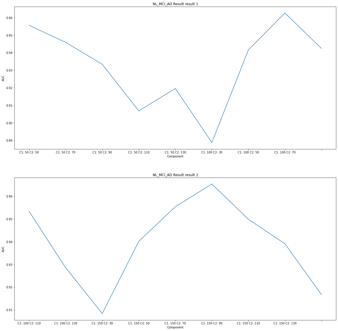
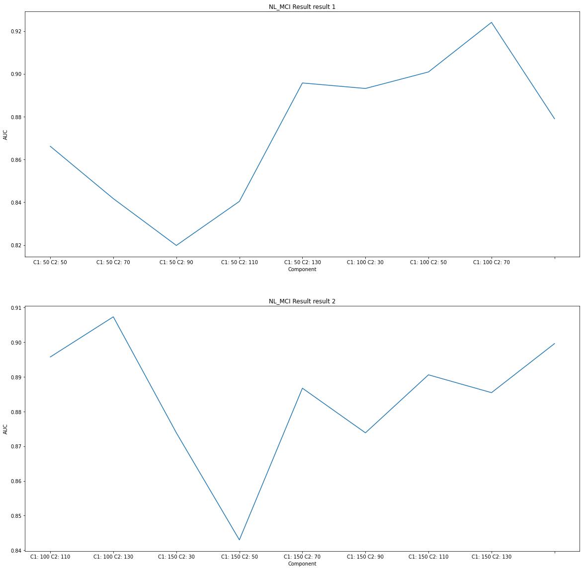
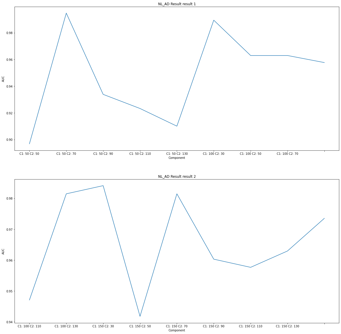
The above figure is when only TestAUC is considered.
Considering only TestAUC, the interpretation of the results is as follows.
As NL_AD is the highest TestAUC, it can be seen that the difference between SNPs and MRI between NL and AD is severe. (You can classify well in the model.)
In addition, it can be seen that NL_MCI_AD has three categories, and distinguishes better than NL_MCI.
Therefore, it can be seen that NL_MCI does not differ much compared to the difference of other subjects.
Component Select Result
Looking at AUC.txt File to select the component considering not only TestAUC but also TrainingAUC and overfitting, the results are as follows.
NL_MCI
Component1: 50 Component2: 30 Train_AUC: 0.883812881097561 Test_AUC: 0.8661518661518661
Component1: 50 Component2: 50 Train_AUC: 0.8991202997967478 Test_AUC: 0.8416988416988418
Component1: 50 Component2: 70 Train_AUC: 0.9104103150406503 Test_AUC: 0.8198198198198198
Component1: 50 Component2: 90 Train_AUC: 0.9143959603658537 Test_AUC: 0.8404118404118404
Component1: 50 Component2: 110 Train_AUC: 0.9299892022357725 Test_AUC: 0.8957528957528957
Component1: 50 Component2: 130 Train_AUC: 0.9432799796747967 Test_AUC: 0.8931788931788931
Component1: 100 Component2: 30 Train_AUC: 0.8692676575203252 Test_AUC: 0.9009009009009009
Component1: 100 Component2: 50 Train_AUC: 0.9153328252032521 Test_AUC: 0.924066924066924
Component1: 100 Component2: 70 Train_AUC: 0.9275438262195121 Test_AUC: 0.879021879021879
Component1: 100 Component2: 90 Train_AUC: 0.9336255081300813 Test_AUC: 0.8957528957528957
Component1: 100 Component2: 110 Train_AUC: 0.9349752286585366 Test_AUC: 0.9073359073359073
Component1: 100 Component2: 130 Train_AUC: 0.9596989329268292 Test_AUC: 0.8738738738738739
Component1: 150 Component2: 30 Train_AUC: 0.8568819867886178 Test_AUC: 0.842985842985843
Component1: 150 Component2: 50 Train_AUC: 0.9150470020325203 Test_AUC: 0.8867438867438867
Component1: 150 Component2: 70 Train_AUC: 0.9200012703252032 Test_AUC: 0.8738738738738738
Component1: 150 Component2: 90 Train_AUC: 0.9147135416666666 Test_AUC: 0.8906048906048906
Component1: 150 Component2: 110 Train_AUC: 0.919969512195122 Test_AUC: 0.8854568854568854
Component1: 150 Component2: 130 Train_AUC: 0.9417873475609756 Test_AUC: 0.8996138996138996
Componet1: 100, Component2: 110 is roughly 90% AUC, so select these components
NL_AD
Component1: 50 Component2: 30 Train_AUC: 0.9217397186147186 Test_AUC: 0.8968253968253969
Component1: 50 Component2: 50 Train_AUC: 0.9416599025974026 Test_AUC: 0.9947089947089947
Component1: 50 Component2: 70 Train_AUC: 0.9539705086580087 Test_AUC: 0.9338624338624338
Component1: 50 Component2: 90 Train_AUC: 0.9687161796536796 Test_AUC: 0.9232804232804233
Component1: 50 Component2: 110 Train_AUC: 0.9793357683982684 Test_AUC: 0.91005291005291
Component1: 50 Component2: 130 Train_AUC: 0.9810944264069265 Test_AUC: 0.9894179894179895
Component1: 100 Component2: 30 Train_AUC: 0.9037472943722943 Test_AUC: 0.9629629629629629
Component1: 100 Component2: 50 Train_AUC: 0.9573525432900433 Test_AUC: 0.9629629629629629
Component1: 100 Component2: 70 Train_AUC: 0.9589082792207793 Test_AUC: 0.9576719576719577
Component1: 100 Component2: 90 Train_AUC: 0.9566084956709956 Test_AUC: 0.9470899470899471
Component1: 100 Component2: 110 Train_AUC: 0.9690882034632036 Test_AUC: 0.9814814814814815
Component1: 100 Component2: 130 Train_AUC: 0.9804180194805194 Test_AUC: 0.9841269841269842
Component1: 150 Component2: 30 Train_AUC: 0.9321225649350651 Test_AUC: 0.9417989417989419
Component1: 150 Component2: 50 Train_AUC: 0.9437229437229437 Test_AUC: 0.9814814814814815
Component1: 150 Component2: 70 Train_AUC: 0.9605316558441558 Test_AUC: 0.9603174603174603
Component1: 150 Component2: 90 Train_AUC: 0.9536661255411255 Test_AUC: 0.9576719576719577
Component1: 150 Component2: 110 Train_AUC: 0.981364989177489 Test_AUC: 0.962962962962963
Component1: 150 Component2: 130 Train_AUC: 0.9835294913419913 Test_AUC: 0.9735449735449735
Componet1: 100, Component2: 130 is roughly 98% AUC, so select these components
NL_MCI_AD
Component1: 50 Component2: 30 Train_AUC: 0.8917560637119589 Test_AUC: 0.9556090776035499
Component1: 50 Component2: 50 Train_AUC: 0.8942808325412073 Test_AUC: 0.9458784931603218
Component1: 50 Component2: 70 Train_AUC: 0.8940696897938386 Test_AUC: 0.9333766476038994
Component1: 50 Component2: 90 Train_AUC: 0.8580887794381642 Test_AUC: 0.9067688259294725
Component1: 50 Component2: 110 Train_AUC: 0.8574048276574779 Test_AUC: 0.9195739974122712
Component1: 50 Component2: 130 Train_AUC: 0.8678200072794825 Test_AUC: 0.8887550070129575
Component1: 100 Component2: 30 Train_AUC: 0.8888001715044882 Test_AUC: 0.9416173177249295
Component1: 100 Component2: 50 Train_AUC: 0.9105276365239678 Test_AUC: 0.962642591279769
Component1: 100 Component2: 70 Train_AUC: 0.9179021591222192 Test_AUC: 0.9423887836755706
Component1: 100 Component2: 90 Train_AUC: 0.9115219838883878 Test_AUC: 0.9533000798080332
Component1: 100 Component2: 110 Train_AUC: 0.9208245185468789 Test_AUC: 0.9285001727619427
Component1: 100 Component2: 130 Train_AUC: 0.9199563389324773 Test_AUC: 0.908375006426084
Component1: 150 Component2: 30 Train_AUC: 0.8948831886990574 Test_AUC: 0.9401646660818933
Component1: 150 Component2: 50 Train_AUC: 0.9243037444427419 Test_AUC: 0.9553980869592414
Component1: 150 Component2: 70 Train_AUC: 0.9187994630651174 Test_AUC: 0.9654132391935316
Component1: 150 Component2: 90 Train_AUC: 0.9296245622346508 Test_AUC: 0.9498550965639918
Component1: 150 Component2: 110 Train_AUC: 0.9382726920533783 Test_AUC: 0.9390808577136466
Component1: 150 Component2: 130 Train_AUC: 0.9424287799177277 Test_AUC: 0.9166700155158454
Componet1: 150, Component2: 110 is roughly 93% AUC, so select these components
Fixed Component, changed Alpha of LossFunction
The number of components was determined through the above training.
Therefore, while adjusting the Alpha value, the focus is on improving the performance of the model. (In the case of Component Select above, it is the result of training each Alpha as 1,1.)
Each proceeds in the following order.
Fix the ROI’s Alpha to 1 and check the value while changing the Alpha of the SNPs.
Check the Alpha value of the maximum AUC of SNPS, fix the Alpha value, and change the Alpha value of the ROI.
Alpha2 Change
1
2
3
4
5
6
7
8
9
10
11
12
13
14
15
16
17
18
19
20
21
22
23
24
25
26
27
28
29
30
31
32
33
34
35
36
37
38
39
40
41
42
43
44
45
46
47
48
49
50
51
52
53
54
# File Path
subject = ['NL_MCI','NL_AD','NL_MCI_AD']
file_path = ['./data/'+subject[0]+'_Data/', './data/'+subject[1]+'_Data/', './data/'+subject[2]+'_Data/']

# Hyperparameter
max_iter = 20000
tol = 1e-7
alpha = [0.001, 0.01, 0.1, 1, 10]

# SNP Result List
nl_mci_list_snp = []
nl_ad_list_snp = []
nl_mci_ad_list_snp = []

print('Alpha2 Change\n')

for i,f in enumerate(file_path):
    # Component Select Result Write
    directory = f+'Alpha2_Change'
    if not os.path.exists(directory):
        os.makedirs(directory)

    aucfile = open(directory+'/auc.txt','a')


    # du1: Component 1, du2: Component 2
    for a in alpha:
        print(subject[i]+' Trainning '+"Alpha2: "+str(a))

        # NL_MCI => Component1: 100, Component2: 110
        if i == 0:
            # SNP Alpha Change => alpha2 Change
            train_auc_1,test_auc_1 = train(max_iter,tol,f,100,110,alpha1=1,alpha2=a)
            nl_mci_list_snp.append(test_auc_1)

        # NL_AD => Component1: 100, Component2: 130
        elif i == 1:
            # SNP Alpha Change => alpha2 Change
            train_auc_1,test_auc_1 = train(max_iter,tol,f,100,130,alpha1=1,alpha2=a)
            nl_ad_list_snp.append(test_auc_1)

        # NL_MCI_AD => Component1: 150, Component2: 110
        else:
            # SNP Alpha Change => alpha2 Change
            train_auc_1,test_auc_1 = train(max_iter,tol,f,150,110,alpha1=1,alpha2=a,NL_MCI_AD=True)
            nl_mci_ad_list_snp.append(test_auc_1)


        # Write Result
        aucfile.write("Alpha1: %s Alpha2: %s Train_AUC: %s Test_AUC: %s\n"%(str(1),str(a),str(train_auc_1),str(test_auc_1)))

        print('Model Test: ',test_auc_1,'\n\n')

    aucfile.close()
1
2
3
4
5
6
7
8
9
10
11
12
13
14
15
16
17
18
19
20
21
22
23
24
25
26
27
28
29
30
31
32
33
34
35
36
37
38
39
40
41
42
43
44
45
46
47
48
49
50
51
52
53
54
55
56
57
58
59
60
61
62
63
64
65
66
67
68
69
70
71
72
73
74
75
76
77
78
79
80
81
82
83
84
85
86
87
88
89
90
91
92
93
94
95
96
97
98
99
100
101
102
103
104
105
106
107
108
109
110
111
112
113
114
115
116
117
118
119
120
121
122
123
124
125
126
127
128
129
130
131
132
133
134
135
136
137
138
139
140
141
142
143
144
145
146
147
148
149
150
151
152
153
154
155
156
157
158
159
160
161
162
163
164
165
166
167
168
169
170
171
172
173
174
175
176
177
178
179
180
181
182
183
184
185
186
187
188
189
190
191
192
193
194
195
196
197
198
199
200
201
202
203
204
205
206
207
208
209
210
211
212
213
214
215
216
217
218
219
220
221
222
223
224
225
226
227
228
229
230
231
232
233
234
Alpha2 Change

NL_MCI Trainning Alpha2: 0.001
Iteration:  0  Train_AUC: 0.5084000254065041
Label:  tensor([[1., 1., 1., 0., 1.]], dtype=torch.float64)
Model Prediction:  tensor([[0.4870, 0.5320, 0.5468, 0.4996, 0.5306]], dtype=torch.float64)

Iteration:  5000  Train_AUC: 0.7950171493902439
Label:  tensor([[1., 1., 1., 0., 1.]], dtype=torch.float64)
Model Prediction:  tensor([[0.5673, 0.7257, 0.6259, 0.3227, 0.6208]], dtype=torch.float64)

Iteration:  10000  Train_AUC: 0.8137385670731707
Label:  tensor([[1., 1., 1., 0., 1.]], dtype=torch.float64)
Model Prediction:  tensor([[0.4988, 0.6817, 0.7700, 0.3318, 0.7372]], dtype=torch.float64)

Iteration:  15000  Train_AUC: 0.8504033282520325
Label:  tensor([[1., 1., 1., 0., 1.]], dtype=torch.float64)
Model Prediction:  tensor([[0.8513, 0.3907, 0.7619, 0.1684, 0.8806]], dtype=torch.float64)

Iteration:  20000  Train_AUC: 0.8799383892276422
Label:  tensor([[1., 1., 1., 0., 1.]], dtype=torch.float64)
Model Prediction:  tensor([[0.9040, 0.3237, 0.9431, 0.1457, 0.9767]], dtype=torch.float64)

Model Test:  0.6396396396396397


...


NL_MCI Trainning Alpha2: 10
Iteration:  0  Train_AUC: 0.5456999491869918
Label:  tensor([[1., 1., 1., 0., 1.]], dtype=torch.float64)
Model Prediction:  tensor([[0.5133, 0.5182, 0.5549, 0.5237, 0.5141]], dtype=torch.float64)

Iteration:  5000  Train_AUC: 0.9128715701219512
Label:  tensor([[1., 1., 1., 0., 1.]], dtype=torch.float64)
Model Prediction:  tensor([[0.5254, 0.8500, 0.5955, 0.5361, 0.9742]], dtype=torch.float64)

Iteration:  10000  Train_AUC: 0.9314500762195121
Label:  tensor([[1., 1., 1., 0., 1.]], dtype=torch.float64)
Model Prediction:  tensor([[0.9528, 0.9080, 0.7225, 0.2458, 0.9805]], dtype=torch.float64)

Iteration:  15000  Train_AUC: 0.9416920731707316
Label:  tensor([[1., 1., 1., 0., 1.]], dtype=torch.float64)
Model Prediction:  tensor([[0.9519, 0.8791, 0.9169, 0.2298, 0.9950]], dtype=torch.float64)

Iteration:  20000  Train_AUC: 0.9443438770325202
Label:  tensor([[1., 1., 1., 0., 1.]], dtype=torch.float64)
Model Prediction:  tensor([[0.9611, 0.9940, 0.9902, 0.0443, 0.9955]], dtype=torch.float64)

Model Test:  0.8584298584298584


NL_AD Trainning Alpha2: 0.001
Iteration:  0  Train_AUC: 0.473045183982684
Label:  tensor([[1., 0., 1., 1., 0.]], dtype=torch.float64)
Model Prediction:  tensor([[0.4929, 0.5177, 0.5146, 0.5509, 0.5233]], dtype=torch.float64)

Iteration:  5000  Train_AUC: 0.9358766233766234
Label:  tensor([[1., 0., 1., 1., 0.]], dtype=torch.float64)
Model Prediction:  tensor([[0.7338, 0.3033, 0.4879, 0.6179, 0.2422]], dtype=torch.float64)

Iteration:  10000  Train_AUC: 0.9543425324675325
Label:  tensor([[1., 0., 1., 1., 0.]], dtype=torch.float64)
Model Prediction:  tensor([[0.7915, 0.0944, 0.6837, 0.8387, 0.1346]], dtype=torch.float64)

Iteration:  15000  Train_AUC: 0.9739583333333333
Label:  tensor([[1., 0., 1., 1., 0.]], dtype=torch.float64)
Model Prediction:  tensor([[0.8863, 0.0844, 0.9035, 0.8280, 0.1265]], dtype=torch.float64)

Iteration:  20000  Train_AUC: 0.9835633116883117
Label:  tensor([[1., 0., 1., 1., 0.]], dtype=torch.float64)
Model Prediction:  tensor([[0.7575, 0.1043, 0.8985, 0.9755, 0.1173]], dtype=torch.float64)

Model Test:  0.9285714285714285


...


NL_AD Trainning Alpha2: 10
Iteration:  0  Train_AUC: 0.49354031385281383
Label:  tensor([[1., 0., 1., 1., 0.]], dtype=torch.float64)
Model Prediction:  tensor([[0.5460, 0.5389, 0.5337, 0.5276, 0.5383]], dtype=torch.float64)

Iteration:  5000  Train_AUC: 0.9436891233766234
Label:  tensor([[1., 0., 1., 1., 0.]], dtype=torch.float64)
Model Prediction:  tensor([[0.7336, 0.0541, 0.8301, 0.7937, 0.2784]], dtype=torch.float64)

Iteration:  10000  Train_AUC: 0.9714894480519481
Label:  tensor([[1., 0., 1., 1., 0.]], dtype=torch.float64)
Model Prediction:  tensor([[0.9027, 0.0256, 0.9006, 0.8147, 0.3772]], dtype=torch.float64)

Iteration:  15000  Train_AUC: 0.9734172077922079
Label:  tensor([[1., 0., 1., 1., 0.]], dtype=torch.float64)
Model Prediction:  tensor([[9.2546e-01, 2.9856e-04, 8.4947e-01, 9.0602e-01, 1.0299e-01]],
       dtype=torch.float64)

Iteration:  20000  Train_AUC: 0.9829545454545454
Label:  tensor([[1., 0., 1., 1., 0.]], dtype=torch.float64)
Model Prediction:  tensor([[0.9660, 0.0024, 0.8637, 0.9935, 0.0460]], dtype=torch.float64)

Model Test:  0.9497354497354498


NL_MCI_AD Trainning Alpha2: 0.001
Iteration:  0  Train_AUC: 0.5241661392236404
Label:  tensor([[0., 0., 1.],
        [0., 1., 0.],
        [1., 0., 0.],
        [0., 0., 1.],
        [0., 1., 0.]], dtype=torch.float64)
Model Prediction:  tensor([[0.3434, 0.3415, 0.3151],
        [0.3532, 0.3214, 0.3253],
        [0.3289, 0.3366, 0.3345],
        [0.3117, 0.3516, 0.3367],
        [0.3297, 0.3457, 0.3246]], dtype=torch.float64)

Iteration:  5000  Train_AUC: 0.772101386117377
Label:  tensor([[0., 0., 1.],
        [0., 1., 0.],
        [1., 0., 0.],
        [0., 0., 1.],
        [0., 1., 0.]], dtype=torch.float64)
Model Prediction:  tensor([[0.2638, 0.4724, 0.2637],
        [0.1820, 0.6244, 0.1936],
        [0.3811, 0.4764, 0.1425],
        [0.2156, 0.5116, 0.2728],
        [0.1879, 0.5445, 0.2676]], dtype=torch.float64)

Iteration:  10000  Train_AUC: 0.8063381384857004
Label:  tensor([[0., 0., 1.],
        [0., 1., 0.],
        [1., 0., 0.],
        [0., 0., 1.],
        [0., 1., 0.]], dtype=torch.float64)
Model Prediction:  tensor([[0.0477, 0.6770, 0.2752],
        [0.2229, 0.7241, 0.0530],
        [0.6638, 0.2149, 0.1213],
        [0.3295, 0.4124, 0.2581],
        [0.0495, 0.4063, 0.5442]], dtype=torch.float64)

Iteration:  15000  Train_AUC: 0.8351770501955134
Label:  tensor([[0., 0., 1.],
        [0., 1., 0.],
        [1., 0., 0.],
        [0., 0., 1.],
        [0., 1., 0.]], dtype=torch.float64)
Model Prediction:  tensor([[0.0293, 0.5507, 0.4199],
        [0.2602, 0.6898, 0.0500],
        [0.5592, 0.4042, 0.0366],
        [0.1017, 0.3900, 0.5083],
        [0.0283, 0.6855, 0.2861]], dtype=torch.float64)

Iteration:  20000  Train_AUC: 0.8398854278641306
Label:  tensor([[0., 0., 1.],
        [0., 1., 0.],
        [1., 0., 0.],
        [0., 0., 1.],
        [0., 1., 0.]], dtype=torch.float64)
Model Prediction:  tensor([[0.0203, 0.4761, 0.5037],
        [0.1021, 0.7450, 0.1528],
        [0.3773, 0.6183, 0.0043],
        [0.1155, 0.4983, 0.3862],
        [0.1189, 0.4211, 0.4599]], dtype=torch.float64)

Model Test:  0.7171091736824867


...


NL_MCI_AD Trainning Alpha2: 10
Iteration:  0  Train_AUC: 0.479055959636427
Label:  tensor([[0., 0., 1.],
        [0., 1., 0.],
        [1., 0., 0.],
        [0., 0., 1.],
        [0., 1., 0.]], dtype=torch.float64)
Model Prediction:  tensor([[0.3114, 0.3413, 0.3473],
        [0.3049, 0.3702, 0.3249],
        [0.3402, 0.3361, 0.3237],
        [0.3507, 0.3157, 0.3336],
        [0.3471, 0.3353, 0.3176]], dtype=torch.float64)

Iteration:  5000  Train_AUC: 0.9086936850103967
Label:  tensor([[0., 0., 1.],
        [0., 1., 0.],
        [1., 0., 0.],
        [0., 0., 1.],
        [0., 1., 0.]], dtype=torch.float64)
Model Prediction:  tensor([[0.4419, 0.3162, 0.2420],
        [0.0528, 0.9065, 0.0407],
        [0.5462, 0.2958, 0.1579],
        [0.4779, 0.3076, 0.2145],
        [0.2312, 0.5147, 0.2541]], dtype=torch.float64)

Iteration:  10000  Train_AUC: 0.8922012026255879
Label:  tensor([[0., 0., 1.],
        [0., 1., 0.],
        [1., 0., 0.],
        [0., 0., 1.],
        [0., 1., 0.]], dtype=torch.float64)
Model Prediction:  tensor([[0.3993, 0.1141, 0.4866],
        [0.0175, 0.8917, 0.0908],
        [0.9941, 0.0029, 0.0030],
        [0.2125, 0.3759, 0.4116],
        [0.1900, 0.7143, 0.0957]], dtype=torch.float64)

Iteration:  15000  Train_AUC: 0.9069446962469954
Label:  tensor([[0., 0., 1.],
        [0., 1., 0.],
        [1., 0., 0.],
        [0., 0., 1.],
        [0., 1., 0.]], dtype=torch.float64)
Model Prediction:  tensor([[0.1289, 0.2795, 0.5916],
        [0.0086, 0.6436, 0.3479],
        [0.9801, 0.0148, 0.0051],
        [0.2996, 0.6246, 0.0758],
        [0.0592, 0.8564, 0.0844]], dtype=torch.float64)

Iteration:  20000  Train_AUC: 0.9149436564531449
Label:  tensor([[0., 0., 1.],
        [0., 1., 0.],
        [1., 0., 0.],
        [0., 0., 1.],
        [0., 1., 0.]], dtype=torch.float64)
Model Prediction:  tensor([[8.4872e-04, 1.8102e-02, 9.8105e-01],
        [1.9905e-02, 8.9815e-01, 8.1941e-02],
        [9.8546e-01, 3.0868e-03, 1.1458e-02],
        [4.1686e-01, 5.3261e-01, 5.0528e-02],
        [8.0123e-02, 8.5884e-01, 6.1038e-02]], dtype=torch.float64)

Model Test:  0.9167125713867823
Visualization Change Alpha
1
2
3
4
5
6
7
8
9
10
11
12
13
14
def component_select_plot(alpha,result1,title,label):
    x_real = alpha
    x = np.arange(len(x_real))

    plt.xlabel('Alpha')
    plt.ylabel('AUC')
    plt.title('{} Change Alpha'.format(title))

    plt.xticks(x,x_real)

    plt.plot(x,result1,label=label)
    plt.legend()

    plt.show()
Alpha2 Change Visualization
1
2
3
# NL_MCI Result Visualization
title = subject[0]
component_select_plot(alpha,nl_mci_list_snp,title,'SNP')
1
2
3
# NL_AD Result Visualization
title = subject[1]
component_select_plot(alpha,nl_ad_list_snp,title,'SNP')
1
2
3
# NL_MCI_AD Result Visualization
title = subject[2]
component_select_plot(alpha,nl_mci_ad_list_snp,title,'SNP')
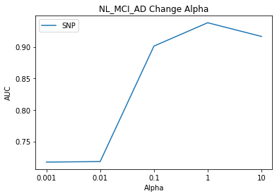
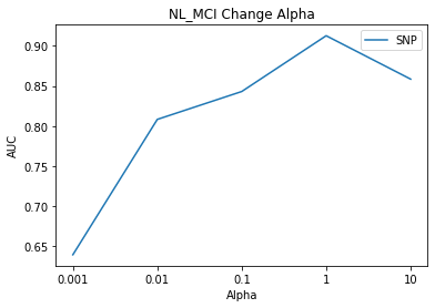
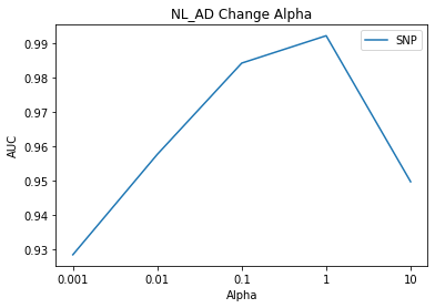
The result of the alpha 2 change is the highest AUC when value is 1.
Now Alpha2 is fixed as 1 and we change the value of Alpha1 to see the result.
Alpha1 Change
1
2
3
4
5
6
7
8
9
10
11
12
13
14
15
16
17
18
19
20
21
22
23
24
25
26
27
28
29
30
31
32
33
34
35
36
37
38
39
40
41
42
43
44
45
46
# ROI Result List
nl_mci_list_roi = []
nl_ad_list_roi = []
nl_mci_ad_list_roi = []
print('Alpha1 Change\n')
for i,f in enumerate(file_path):
# Component Select Result Write
directory = f+'Alpha1_Change'
if not os.path.exists(directory):
os.makedirs(directory)
aucfile = open(directory+'/auc.txt','a')
# du1: Component 1, du2: Component 2
for a in alpha:
print(subject[i]+' Trainning '+"Alpha1: "+str(a))
# NL_MCI => Component1: 100, Component2: 110
if i == 0:
# ROI Alpha Change => alpha1 Change
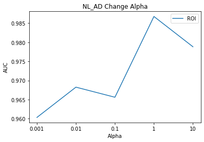
train_auc_2,test_auc_2 = train(max_iter,tol,f,100,110,alpha1=a,alpha2=1)
nl_mci_list_roi.append(test_auc_2)
# NL_AD => Component1: 100, Component2: 130
elif i == 1:
# ROI Alpha Change => alpha1 Change
train_auc_2,test_auc_2 = train(max_iter,tol,f,100,130,alpha1=a,alpha2=1)
nl_ad_list_roi.append(test_auc_2)
# NL_MCI_AD => Component1: 150, Component2: 110
else:
# ROI Alpha Change => alpha1 Change
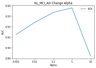
train_auc_2,test_auc_2 = train(max_iter,tol,f,150,110,alpha1=a,alpha2=1,NL_MCI_AD=True)
nl_mci_ad_list_roi.append(test_auc_2)
# Write Result
aucfile.write("Alpha1: %s Alpha2: %s Train_AUC: %s Test_AUC: %s\n"%(str(a),str(1),str(train_auc_2),str(test_auc_2)))
print('Model Test: ',test_auc_2,'\n\n')
aucfile.close()
1
2
3
4
5
6
7
8
9
10
11
12
13
14
15
16
17
18
19
20
21
22
23
24
25
26
27
28
29
30
31
32
33
34
35
36
37
38
39
40
41
42
43
44
45
46
47
48
49
50
51
52
53
54
55
56
57
58
59
60
61
62
63
64
65
66
67
68
69
70
71
72
73
74
75
76
77
78
79
80
81
82
83
84
85
86
87
88
89
90
91
92
93
94
95
96
97
98
99
100
101
102
103
104
105
106
107
108
109
110
111
112
113
114
115
116
117
118
119
120
121
122
123
124
125
126
127
128
129
130
131
132
133
134
135
136
137
138
139
140
141
142
143
144
145
146
147
148
149
150
151
152
153
154
155
156
157
158
159
160
161
162
163
164
165
166
167
168
169
170
171
172
173
174
175
176
177
178
179
180
181
182
183
184
185
186
187
188
189
190
191
192
193
194
195
196
197
198
199
200
201
202
203
204
205
206
207
208
209
210
211
212
213
214
215
216
217
218
219
220
221
222
223
224
225
226
227
228
229
230
231
232
233
Alpha1 Change

NL_MCI Trainning Alpha1: 0.001
Iteration:  0  Train_AUC: 0.46189024390243905
Label:  tensor([[1., 1., 1., 0., 1.]], dtype=torch.float64)
Model Prediction:  tensor([[0.5013, 0.5380, 0.4869, 0.5192, 0.5228]], dtype=torch.float64)

Iteration:  5000  Train_AUC: 0.9123793191056911
Label:  tensor([[1., 1., 1., 0., 1.]], dtype=torch.float64)
Model Prediction:  tensor([[0.8507, 0.8599, 0.7693, 0.2911, 0.9377]], dtype=torch.float64)

Iteration:  10000  Train_AUC: 0.939723069105691
Label:  tensor([[1., 1., 1., 0., 1.]], dtype=torch.float64)
Model Prediction:  tensor([[0.9888, 0.8912, 0.5109, 0.0726, 0.9863]], dtype=torch.float64)

Iteration:  15000  Train_AUC: 0.9540936229674797
Label:  tensor([[1., 1., 1., 0., 1.]], dtype=torch.float64)
Model Prediction:  tensor([[0.9881, 0.9853, 0.9282, 0.1881, 0.9982]], dtype=torch.float64)

Iteration:  20000  Train_AUC: 0.9537125254065041
Label:  tensor([[1., 1., 1., 0., 1.]], dtype=torch.float64)
Model Prediction:  tensor([[0.9846, 0.9386, 0.7891, 0.2020, 0.9819]], dtype=torch.float64)

Model Test:  0.9305019305019305


...


NL_MCI Trainning Alpha1: 10
Iteration:  0  Train_AUC: 0.4700044461382114
Label:  tensor([[1., 1., 1., 0., 1.]], dtype=torch.float64)
Model Prediction:  tensor([[0.5348, 0.5401, 0.5137, 0.5311, 0.5382]], dtype=torch.float64)

Iteration:  5000  Train_AUC: 0.912379319105691
Label:  tensor([[1., 1., 1., 0., 1.]], dtype=torch.float64)
Model Prediction:  tensor([[0.8632, 0.7454, 0.8196, 0.3023, 0.8400]], dtype=torch.float64)

Iteration:  10000  Train_AUC: 0.9391990599593497
Label:  tensor([[1., 1., 1., 0., 1.]], dtype=torch.float64)
Model Prediction:  tensor([[0.3567, 0.9535, 0.9135, 0.1334, 0.9897]], dtype=torch.float64)

Iteration:  15000  Train_AUC: 0.933371443089431
Label:  tensor([[1., 1., 1., 0., 1.]], dtype=torch.float64)
Model Prediction:  tensor([[0.5743, 0.9870, 0.9183, 0.0711, 0.9955]], dtype=torch.float64)

Iteration:  20000  Train_AUC: 0.9241298272357725
Label:  tensor([[1., 1., 1., 0., 1.]], dtype=torch.float64)
Model Prediction:  tensor([[0.8013, 0.9913, 0.9815, 0.0251, 0.9938]], dtype=torch.float64)

Model Test:  0.8082368082368082


NL_AD Trainning Alpha1: 0.001
Iteration:  0  Train_AUC: 0.4284699675324675
Label:  tensor([[1., 0., 1., 1., 0.]], dtype=torch.float64)
Model Prediction:  tensor([[0.5415, 0.5273, 0.5399, 0.4856, 0.5433]], dtype=torch.float64)

Iteration:  5000  Train_AUC: 0.9222808441558441
Label:  tensor([[1., 0., 1., 1., 0.]], dtype=torch.float64)
Model Prediction:  tensor([[0.5702, 0.1960, 0.4800, 0.8268, 0.2607]], dtype=torch.float64)

Iteration:  10000  Train_AUC: 0.9541734307359307
Label:  tensor([[1., 0., 1., 1., 0.]], dtype=torch.float64)
Model Prediction:  tensor([[0.6639, 0.0435, 0.5292, 0.5840, 0.0905]], dtype=torch.float64)

Iteration:  15000  Train_AUC: 0.9823119588744589
Label:  tensor([[1., 0., 1., 1., 0.]], dtype=torch.float64)
Model Prediction:  tensor([[0.3119, 0.0079, 0.9226, 0.6301, 0.1056]], dtype=torch.float64)

Iteration:  20000  Train_AUC: 0.9826163419913421
Label:  tensor([[1., 0., 1., 1., 0.]], dtype=torch.float64)
Model Prediction:  tensor([[0.9802, 0.0174, 0.9623, 0.3147, 0.3073]], dtype=torch.float64)

Model Test:  0.9603174603174602


...


NL_AD Trainning Alpha1: 10
Iteration:  0  Train_AUC: 0.49171401515151514
Label:  tensor([[1., 0., 1., 1., 0.]], dtype=torch.float64)
Model Prediction:  tensor([[0.4750, 0.5271, 0.5333, 0.5371, 0.5630]], dtype=torch.float64)

Iteration:  5000  Train_AUC: 0.9650974025974025
Label:  tensor([[1., 0., 1., 1., 0.]], dtype=torch.float64)
Model Prediction:  tensor([[0.5915, 0.0650, 0.6997, 0.6951, 0.3369]], dtype=torch.float64)

Iteration:  10000  Train_AUC: 0.9704410173160174
Label:  tensor([[1., 0., 1., 1., 0.]], dtype=torch.float64)
Model Prediction:  tensor([[0.9709, 0.0461, 0.8265, 0.9857, 0.1146]], dtype=torch.float64)

Iteration:  15000  Train_AUC: 0.9717261904761905
Label:  tensor([[1., 0., 1., 1., 0.]], dtype=torch.float64)
Model Prediction:  tensor([[0.9353, 0.0136, 0.9735, 0.9807, 0.0925]], dtype=torch.float64)

Iteration:  20000  Train_AUC: 0.9858292748917749
Label:  tensor([[1., 0., 1., 1., 0.]], dtype=torch.float64)
Model Prediction:  tensor([[0.9720, 0.1999, 0.9712, 0.9817, 0.0293]], dtype=torch.float64)

Model Test:  0.9788359788359788


NL_MCI_AD Trainning Alpha1: 0.001
Iteration:  0  Train_AUC: 0.49128345421235303
Label:  tensor([[0., 0., 1.],
        [0., 1., 0.],
        [1., 0., 0.],
        [0., 0., 1.],
        [0., 1., 0.]], dtype=torch.float64)
Model Prediction:  tensor([[0.3239, 0.3407, 0.3355],
        [0.3188, 0.3649, 0.3163],
        [0.3369, 0.3608, 0.3024],
        [0.3504, 0.3069, 0.3426],
        [0.3155, 0.3428, 0.3417]], dtype=torch.float64)

Iteration:  5000  Train_AUC: 0.9041970598828334
Label:  tensor([[0., 0., 1.],
        [0., 1., 0.],
        [1., 0., 0.],
        [0., 0., 1.],
        [0., 1., 0.]], dtype=torch.float64)
Model Prediction:  tensor([[0.4093, 0.3520, 0.2387],
        [0.1022, 0.7813, 0.1166],
        [0.4754, 0.4332, 0.0914],
        [0.1341, 0.6965, 0.1694],
        [0.3087, 0.5798, 0.1114]], dtype=torch.float64)

Iteration:  10000  Train_AUC: 0.8954521823275675
Label:  tensor([[0., 0., 1.],
        [0., 1., 0.],
        [1., 0., 0.],
        [0., 0., 1.],
        [0., 1., 0.]], dtype=torch.float64)
Model Prediction:  tensor([[0.1157, 0.7340, 0.1503],
        [0.0358, 0.8826, 0.0816],
        [0.8500, 0.0921, 0.0578],
        [0.2371, 0.6914, 0.0715],
        [0.3302, 0.5378, 0.1320]], dtype=torch.float64)

Iteration:  15000  Train_AUC: 0.8892645342869517
Label:  tensor([[0., 0., 1.],
        [0., 1., 0.],
        [1., 0., 0.],
        [0., 0., 1.],
        [0., 1., 0.]], dtype=torch.float64)
Model Prediction:  tensor([[0.6378, 0.0339, 0.3283],
        [0.0329, 0.9105, 0.0566],
        [0.9843, 0.0062, 0.0096],
        [0.0145, 0.9149, 0.0707],
        [0.0428, 0.9282, 0.0290]], dtype=torch.float64)

Iteration:  20000  Train_AUC: 0.9259148518791598
Label:  tensor([[0., 0., 1.],
        [0., 1., 0.],
        [1., 0., 0.],
        [0., 0., 1.],
        [0., 1., 0.]], dtype=torch.float64)
Model Prediction:  tensor([[1.9603e-01, 1.7658e-02, 7.8631e-01],
        [7.4874e-03, 9.7755e-01, 1.4968e-02],
        [9.9952e-01, 4.4223e-04, 4.1779e-05],
        [2.5844e-01, 6.4709e-01, 9.4474e-02],
        [1.3048e-01, 8.4732e-01, 2.2198e-02]], dtype=torch.float64)

Model Test:  0.9126603442938568


...


NL_MCI_AD Trainning Alpha1: 10
Iteration:  0  Train_AUC: 0.5097526175502312
Label:  tensor([[0., 0., 1.],
        [0., 1., 0.],
        [1., 0., 0.],
        [0., 0., 1.],
        [0., 1., 0.]], dtype=torch.float64)
Model Prediction:  tensor([[0.3396, 0.3426, 0.3178],
        [0.3363, 0.3295, 0.3341],
        [0.3353, 0.3356, 0.3291],
        [0.3505, 0.3128, 0.3367],
        [0.3456, 0.3320, 0.3224]], dtype=torch.float64)

Iteration:  5000  Train_AUC: 0.8066686460256798
Label:  tensor([[0., 0., 1.],
        [0., 1., 0.],
        [1., 0., 0.],
        [0., 0., 1.],
        [0., 1., 0.]], dtype=torch.float64)
Model Prediction:  tensor([[0.1862, 0.4872, 0.3266],
        [0.1533, 0.6716, 0.1751],
        [0.4303, 0.4503, 0.1194],
        [0.3310, 0.3736, 0.2955],
        [0.2584, 0.4943, 0.2474]], dtype=torch.float64)

Iteration:  10000  Train_AUC: 0.9112268511537139
Label:  tensor([[0., 0., 1.],
        [0., 1., 0.],
        [1., 0., 0.],
        [0., 0., 1.],
        [0., 1., 0.]], dtype=torch.float64)
Model Prediction:  tensor([[0.0405, 0.4887, 0.4708],
        [0.3113, 0.4983, 0.1904],
        [0.6285, 0.2453, 0.1263],
        [0.2205, 0.3101, 0.4694],
        [0.1732, 0.5363, 0.2906]], dtype=torch.float64)

Iteration:  15000  Train_AUC: 0.9300076875985904
Label:  tensor([[0., 0., 1.],
        [0., 1., 0.],
        [1., 0., 0.],
        [0., 0., 1.],
        [0., 1., 0.]], dtype=torch.float64)
Model Prediction:  tensor([[0.1079, 0.3015, 0.5906],
        [0.1057, 0.8037, 0.0906],
        [0.8384, 0.1411, 0.0205],
        [0.0579, 0.9079, 0.0342],
        [0.2344, 0.2911, 0.4744]], dtype=torch.float64)

Iteration:  20000  Train_AUC: 0.9337588446051192
Label:  tensor([[0., 0., 1.],
        [0., 1., 0.],
        [1., 0., 0.],
        [0., 0., 1.],
        [0., 1., 0.]], dtype=torch.float64)
Model Prediction:  tensor([[1.5291e-03, 3.2663e-02, 9.6581e-01],
        [2.0231e-01, 6.0693e-01, 1.9076e-01],
        [9.5905e-01, 4.0152e-02, 7.9446e-04],
        [1.5437e-02, 3.4720e-01, 6.3736e-01],
        [4.5573e-02, 7.3962e-01, 2.1480e-01]], dtype=torch.float64)

Model Test:  0.891925043675278
Alpha1 Change Visualization
1
2
3
# NL_MCI Result Visualization
title = subject[0]
component_select_plot(alpha,nl_mci_list_roi,title,'ROI')
1
2
3
# NL_AD Result Visualization
title = subject[1]
component_select_plot(alpha,nl_ad_list_roi,title,'ROI')
1
2
3
# NL_MCI_AD Result Visualization
title = subject[2]
component_select_plot(alpha,nl_mci_ad_list_roi,title,'ROI')
Result
NL_MCI_Model
- Component1: 100
- Component2: 110
- Alpha1: 0.001
- Alpha2: 1
- AUC: 0.93
NL_AD_Model
- Component1: 100
- Component2: 110
- Alpha1: 1
- Alpha2: 1
- AUC: 0.98
NL_MCI_AD_Model
- Component1: 150
- Component2: 110
- Alpha1: 1
- Alpha2: 1
- AUC: 0.93
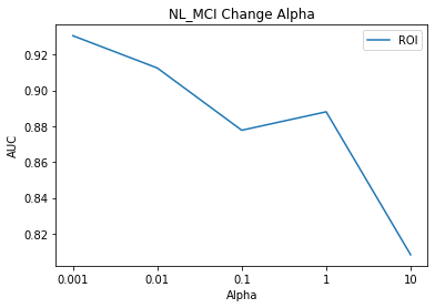
In other models, although the Alpha value was modified, the AUC value was the same, but in the case of the NL_MCI Model, the AUC rose from 90% to 93% due to the change in the Alpha value.
When thinking of AutoEncoder, in the configuration of commonly used Encoder, NL_AD and NL_MCI_AD have the highest values when SNPs and MRI are the same Alpha value, but the highest value is NL_MCI Alpha1: 0.001 (ROI), Alpha2: The best performance was the use of 1 (SNPs).
I think the idea of the paper that judges which modality is important due to the simple ratio is wrong.
Since the number of features of SNPs and MRI is different, the absolute value of loss will also be different.
In addition, how the Encoder extracts features well, and accordingly, the weight of the classification model will be different.
In other words, it is a value that needs to be determined as a learning rate, and it is difficult to think that absolutely any data has more influence on the model.
In order to find out what kind of modality actually affects the classification of patients, it would be an accurate way to find out through CAM techniques.
참조: 원본코드
참조: Multi-Modality Disease Modeling via Collective Deep Matrix Factorization
참조: SVD based initialization: A head start for nonnegative matrix factorization
참조: The Effect of Age Correction on Multivariate Classification in Alzheimer’s Disease, with a Focus on the Characteristics of Incorrectly and Correctly Classified Subjects
참조: A large scale multivariate parallel ICA method reveals novel imaging–genetic relationships for Alzheimer’s disease in the ADNI cohort’s Method
코드에 문제가 있거나 궁금한 점이 있으면 wjddyd66@naver.com으로 Mail을 남겨주세요.
Leave a comment