Paper30. Adversarial Autoencoders

8 minute read

Adversarial Autoencoders

이 Poster는 아래 논문과 Blog들을 참조하여 정리하였다는 것을 먼저 밝힙니다.

Paper: Adversarial Autoencoders
Code:
- (1). bfarzin GitHub
- (2). yoonsanghyu GitHub
참조 Blog: Gorio Learning Blog
Background
- (1). VAE
- (2). GAN

Abstract

In this paper, we propose the “adversarial autoencoder” (AAE), which is a probabilistic autoencoder that uses the recently proposed generative adversarial networks (GAN) to perform variational inference by matching the aggregated posterior of the hidden code vector of the autoencoder with an arbitrary prior distribution.
Matching the aggregated posterior to the prior ensures that generating from any part of prior space results in meaningful samples.
As a result, the decoder of the adversarial autoencoder learns a deep generative model that maps the imposed prior to the data distribution.
We show how the adversarial autoencoder can be used in applications such as semi-supervised classification, disentangling style and content of images, unsupervised clustering, dimensionality reduction and data visualization.
We performed experiments on MNIST, Street View House Numbers and Toronto Face datasets and show that adversarial autoencoders achieve competitive results in generative modeling and semi-supervised classification tasks.

제안하는 AAE (adversarial autoencoder)는 기존의 AE (autoencoder)에 GAN (generative adversarial networks)을 사용하여 arbitrary prior distribution와 aggregated posterior of the hidden code vector of the autoencoder를 일치시키는 새로운 model을 제안한다.
해당 결과로서 prior로서 의미있는 sample을 generation할수 있게 된다.
해당 논문은 이를 증명하기 위하여 여러 Task와 여러 Data에서 결과를 증명하였다.

Introduction

In these approaches the MCMC methods [Boltzmann Machines (RBM), Deep Belief Networks (DBNs) and Deep Boltzmann Machines (DBMs)] compute the gradient of log-likelihood which becomes more imprecise as training progresses.
This is because samples from the Markov Chains are unable to mix between modes fast enough.
In recent years, generative models have been developed that may be trained via direct back-propagation and avoid the difficulties that come with MCMC training.

해당 논문에서는 MCMC methods를 사용하여 log-likelihood의 기울기를 계산하여 direct-backpropagation을 계산하는 것은 inprecise한 결과를 얻는다고 표현하고 있다. (개인적인 해석은 모든 Sample에 대하여 추론할 수 있는 Distribution이 아닌 각각의 해당 몇몇 sample에 맞춰서 model이 Training되어 Overfitting이 발생하게 된다는 의미인 것 같습니다. 이러한 결과는 sample이 매우 적을때나 많을 때 모두 적합하지 않을 것 이라고 판단됩니다.)

이러한 문제점을 해결하기 위하여 Latent Represenation을 Distribution으로서 표현하여 GAN과 VAE는 Direct-Backpropagation문제를 해결하였다.

해당 논문은 이러한 GAN과 VAE를 결합하는 AAE라는 model을 제안한다.
해당 논문의 목적은 Arbitrary prior distribution와 Aggregated posterior를 2개의 목적함수 (Traditional Reconstruction Error Criterion, Adversarial Training Criterion)로서 연결시키는 model을 제안한다.
Encoder가 데이터 분포를 Prior 분포로 변환하는 방법에 대해 학습하고 Decoder는 Imposed Prior를 데이터 분포에 매핑하는 Deep 생성 모델을 학습하게 된다.

Background: Generative Adversarial Networks

GAN을 살펴보게 되면 Generator로 생성된 $G(z)$와 실제 data를 Discriminator $D(z)$로서 서로 구별하지 못하게 하는 것이 목적이다.

위의 그림에서의 의미는 각각 다음과 같다.

검은 점선: 실제 데이터의 분포(Data generating Distribution), $P_{\text{data}}$
녹색 점선: 생성된 데이터의 분포(Discriminator Distribution), $P_g$
파란 점선: 판별자가 데이터의 판별 결과 분포(Generative Distribution), $D(x)$

(a): 처음 시작할 때는 pdata와 pg의 분포는 매우 다른 것을 알 수 있다.

(b), (c): 이러한 상황에서

$$\underset{G}{min} \underset{D}{max}V(D,G) =$$

$$\mathbb{E}_{x\text{~}P_{data}(x)}[logD(x)] + \mathbb{E}_{z\text{~}P_{z}(z)}[log(1 - D(G(z)))]$$

을 학습하다 보면 $D(x)$의 파란점선이 점점 smooth하고 잘 구별하는 Distribution이 만들어 진다.

(d): Trainning의 최종적인 Distribution의 모양은 $P_{\text{data}} = P_g$으로서 $D(x)=\frac{1}{2}$의 값을 가지는 것을 알 수 있다.

자세한 내용은 GAN에 정리되어 있습니다.

Notation

$x$: Data
$z$: Latent representation
$p(z)$: Prior
$q(z|x)$: Encoding distribution
$p(x|z)$: Decoding distribution
$p_d(x)$: Real data distribution
$p(x)$: Model distribution
$p(z)$: Arbitary Prior
$q(z)$: Aggregated Posterior

Adversarial Autoencoders

png

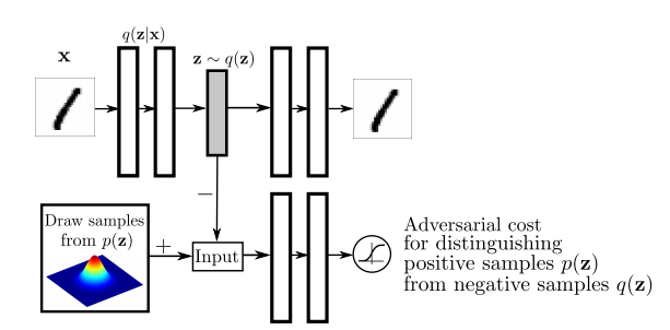
해당 논문에서 먼저 aggregated posterior distribution of $q(z)$ on the hidden code vector of the autoencoder를 아래와 같이 표현한다.

$$q(z) = \int_{x} q(z|x) p_d (x)\, dx$$

위의 Figure를 살펴보게 되면 AAE는 위에서 구한 $q(z)$ (Aggreagted Posterior)와 실제 Prior인 $p(z)$가 비슷해지도록 Discriminator를 통하여 판별하도록 학습된다.
AAE는 SGD를 통하여 다음과 같은 2가지 phase를 통하여 학습된다.

Reconstruction: Encoder와 Decoder가 Input에 대한 Reconstruction할 수 있도록 학습한다.
Regularization: Adversarial Networ를 통하여 $q(z)$와 $p(z)$를 구별하지 못하게 학습한다.

해당 논문에서는 Encoder인 $q(z|x)$에 대하여 다음과 같이 3가지 경우에 대하여 정의하였다.

Deterministic: $p_d(x)$에 의해서 결정되는 Encoder라 생각하게 되면, 기본적인 AutoEncoder의 Encoder와 동일한 형태이다.
Gaussian posterior: $z_i \sim N(\mu_i(x), \sigma_i(x))$라고 가정하게 되면 GAN과 동일한 형태가 되며, 학습하기 위하여 Reparametrization Trick이 필요하게 된다.
Universal approximator posterior: 해당 방법은 Gaussian처럼 fixed된 distribution에서 random noise $\eta$를 sampling하여 $f(x, \eta)$를 평가하는 방법이다. (GAN과 비슷한 방법이다.) 해당 방법은 아래와 같다.

$$q(z|x) = \int_{\eta} q(z|x,\eta) p_{\eta} (\eta)\, d \eta$$

$$q(z) \rightarrow \int_{x} \int_{\eta} q(z|x,\eta) p_d(x) p_{\eta} p_{\eta} (\eta)\, d \eta dx$$

위와 같은 방법으로서 Posterior를 구하면 좋은 점으로는 더 이상 $q(z|x)$가 Gaussian으로서 고정되어야 할 이유도 없어지는 방법이다. 또한, (2) Gaussian posterior처럼 Reparametrization Trick을 거친 form이므로 Encoder에 직접적으로 Back-propataion이 가능하다.

위와같은 3가지의 posterior를 설정하는 방법에서 (1) Deterministic의 방법은 위에서 설명한 Introduction에서의 direct-backpropagation 문제점처럼 “모든 Sample에 대하여 추론할 수 있는 Distribution이 아닌 각각의 해당 몇몇 sample에 맞춰서 model이 Training되어 Overfitting이 발생”한다는 문제점이 있을 수 있을 것 같습니다. 즉, smooth한 $q(z)$를 만들 수 없다는 문제점이 발생하게 됩니다.

하지만 나머지 2개의 문제는 latent representation을 “stochastic”으로서 표현하게 되어 $q(z)$를 smooth하게 만들수 있다는 장점이 생기게 됩니다.

Relationship to Variational Autoencoders

GAN의 Loss Function을 살펴보면 다음과 같습니다.

$$\log p(x) \ge E_{z \sim q(z)} [\log p(x|z)] - D_{KL} (q(z) || p(z|x))$$

위의 수식을 동일하게 전개하면 아래와 같이 표현될 수 있습니다.

$$E_{x \sim p_d(x)} [-\log p(x)] < E_x [E_{q(z|x)} [- \log p(x|z)]] + E_x[\text{KL} (q(z|x) || p(z))]$$

$$E_x [E_{q(z|x)} [- \log p(x|z)]] + E_x[\text{KL} (q(z|x) || p(z))]$$

$$= E_x [E_{q(z|x)} [- \log p(x|z)]] - E_x[\text{H} (q(z|x))] +E_{q(z)}[-\log p(z)]$$

$$=\text{Reconstruction} - \text{Entropy} + \text{CrossEntorpy}(q(z), p(z))$$

VAE의 식을 살펴보게 되면, $q(z)$와 $p(z)$가 비슷한 분포를 가지도록 바로 Crossentropy를 거치는 것을 알 수 있다. 하지만, AAE에서는 이것을 GAN을 사용하여 $p(z), q(z) \rightarrow \text{Latent Representation} (p(z), q(z))$로 Mapping하여 Discriminator가 구별하지 못하도록 학습하는 것을 알 수 있다.

해당 수식만 보았을때, Discriminator를 통하여 Distribution을 맞춰주는 것이 실제로 더 효과가 있는지 알 수 없다. 따라서 해당 논문은 많은 실험을 통하여 VAE와 AAE의 차이를 확인하였다.

png

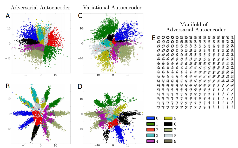
먼저 위의 그림을 살펴보게 되면, Prior인 $z$를 Visualization한 결과이다.
A,C의 경우에는 2차원 Gaussian Distribution으로서 가정하고 학습한 결과이다. 해당 결과를 확인하게 되면, AAE의 경우에는 빈틈이 없지만, VAE의 경우에는 빈 부분이 많도록 학습되는 것을 알 수 있다. 이는 AAE는 Manifold를 잘 포착하여 smooth하게 잘 datapoint들을 포착하였지만, VAE는 일부 Local Region은 파악하지 못한 것을 알 수 있다.

또한, B,D의 경우에는 10개의 2차원 Gaussian Distribution으로서 가정하고 학습한 결과이다. AAE의 결과는 정확한 10개의 Gaussian으로서 분류되는 것을 알 수 있지만, VAE는 부족한 결과를 보여준다.

이러한 결과의 차이는 Loss Funciton을 자세히 살펴보게 되면, VAE는 직접적으로 $\text{CrossEntorpy}(q(z), p(z))$를 수행해야 하므로, Prior의 정확한 분포를 알아야 된다는 단점이 있지만, AAE는 Discriminator로서 추가적인 Distribution을 맞춰줄 수 있으므로 단순히 Prior ($p(z)$)에서 Sampling만 할 수 있으면 된다는 장점이 있다.

Incorporating Label Information in the Adversarial Regularization

“Relationship to Variational Autoencoders” Section의 결과에서 MNIST의 결과 10개의 2차원 Gaussian Distribution으로서 충분히 z를 분류할 수 있다는 것을 알 수 있었다. 이에대하여 Label정보를 넣었을 경우 어떠한 변화가 있는지 확인하기 위하여 해당 model의 Label의 정보를 아래와 같이 추가하여 실험을 진행하였다.

png

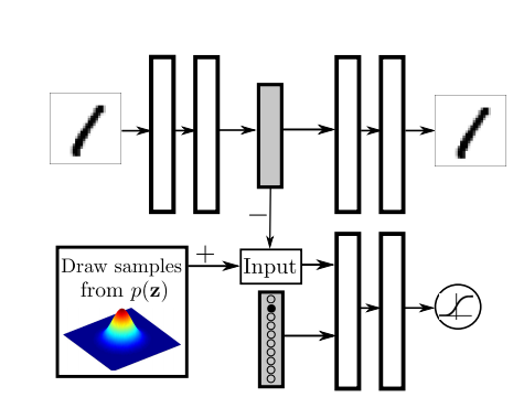
위의 Figure를 보게 되면, 기존의 Input인 $z$외에 Label의 정보를 One-Hot Encoding으로서 추가적으로 넣게 된다. 해당 논문 저자는 이러한 Label정보가 Switch와 같은 역할을 할 것이라고 얘기하고 있다. (실제 Code상에서 concat하여 넣었습니다.)

png

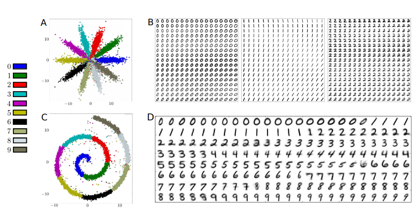
위의 Figure는 실험 결과이다. 먼저 A를 살펴보게 되면, 기존의 Unsupervised Learning으로 학습된 거와 비교하였을때, 확실히 Label의 정보대로 분류가 된것을 알 수 있다.
또한 B를 살펴보게 되면, 같은 Class안에서도 서로 Style이 비슷한 사진끼리 Clustering된 것을 알 수 있다.

마지막으로 Figure C,D는 MNIST는 swiss roll처럼 mapping한 결과이다. (어떻게 swiss roll처럼 mapping하는 지에 대해서는 나와있지 않습니다.) 해당 결과, 0 -> 1뿐만 아니라 다른 Class와 인접한 사진은 흐리고 가운데의 Class의 특징을 대표하는 사진은 뚜렷한 것을 알 수 있다.

Supervised Adversarial Autoencoders

위의 Section의 결과로 알수 있는 사실은 크게 2가지 였다.

Classification정보인 Label을 넣었을 경우, Latent Representation $z$에 충분한 Label정보가 포함되게 학습된다.
하나의 Class안에서도 Style이 각각 존재하며, 비슷한 Style끼리 근접한 Space에 위치한다.

위의 두가지 결과 중 2번째를 좀 더 specific하게 확인하기 위하여 아래와 같은 model로서 구성하고 실험하였다.

png

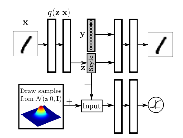
위의 Figure를 살펴보게 되면, z는 15-Dimension Gaussian으로서 가정하고 학습을 실시하였다. 해당 model은 label정보또한 포함하여 Reconstruction을 수행하고, 각각의 Class안에서 Style또한 분류하겠다는 의미이다.

png

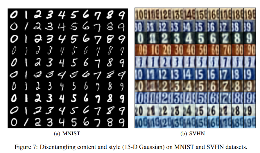
해당 실험결과의 Figure는 위와 같다. (a)를 살펴보게 되면, Class별로 분류할 뿐만 아니라, 각각의 Class별로 Style또한 비슷한 결과를 얻을 수 있는 것을 확인할 수 있다.

해당 논문은 위의 2가지 결과 뿐만 아니라 (1) Semi-Supervised Adversarial Autoencoders, (2) Unsupervised Clustering with Adversarial Autoencoders, (3) Dimensionality Reduction with Adversarial Autoencoders에 대해서도 각각 실험을 하였다. 해당 내용이 궁금하면 해당 논문을 찾아보시길 바란다.

Pytorch Code - Supervised Adversarial Autoencoders

Model

class Encoder(nn.Module):
    def __init__(self):
        super(Encoder, self).__init__()

        self.model = nn.Sequential(
            nn.Linear(int(np.prod(img_shape)), 512),
            nn.LeakyReLU(0.2, inplace=True),
            nn.Linear(512, 512),
            nn.BatchNorm1d(512),
            nn.LeakyReLU(0.2, inplace=True),
            nn.Linear(512, args.latent_dim)
        )

        self.mu = nn.Linear(512, args.latent_dim)
        self.logvar = nn.Linear(512, args.latent_dim)

    def forward(self, img):
        img_flat = img.view(img.shape[0], -1)
        x = self.model(img_flat)
        # mu = self.mu(x)
        # logvar = self.logvar(x)
        # z = reparameterization(mu, logvar)
        return x

class Decoder(nn.Module):
    def __init__(self):
        super(Decoder, self).__init__()

        self.model = nn.Sequential(
            nn.Linear(args.latent_dim + args.n_classes, 512),
            nn.LeakyReLU(0.2, inplace=True),
            nn.Linear(512, 512),
            nn.BatchNorm1d(512),
            nn.LeakyReLU(0.2, inplace=True),
            nn.Linear(512, int(np.prod(img_shape))),
            nn.Tanh(),
        )

    def forward(self, z):
        img_flat = self.model(z)
        img = img_flat.view(img_flat.shape[0], *img_shape)
        return img

class Discriminator(nn.Module):
    def __init__(self):
        super(Discriminator, self).__init__()

        self.model = nn.Sequential(
            nn.Linear(args.latent_dim, 512),
            nn.LeakyReLU(0.2, inplace=True),
            nn.Linear(512, 256),
            nn.LeakyReLU(0.2, inplace=True),
            nn.Linear(256, 1),
            nn.Sigmoid(),
        )

    def forward(self, z):
        validity = self.model(z)
        return validity

Loss Function

$$E_{x \sim p_d(x)} [-\log p(x)] < E_x [E_{q(z|x)} [- \log p(x|z)]] + E_x[\text{KL} (q(z|x) || p(z))]$$

$$= E_x [E_{q(z|x)} [- \log p(x|z)]] - E_x[\text{H} (q(z|x))] +E_{q(z)}[-\log p(z)]$$

$$=\text{Reconstruction} - \text{Entropy} + \text{CrossEntorpy}(q(z), p(z))$$

fake_z: $x \rightarrow q(z|x) \rightarrow z \sim q(z)$
fake_z_cat: $\text{One-Hot-Encoding Label}$
fake_z_concatenate: $\text{Cat}(q(z), \text{One-Hot-Encoding Label})$
decoded_x: $p(x|z)$
reconstruction_loss(decoded_x, x): $E_x [E_{q(z|x)} [- \log p(x|z)]]$
adversarial_loss(validity_fake_z, valid): $\text{CrossEntorpy}(q(z), p(z))$
D_loss = 0.5*(real_loss + fake_loss): $\text{GAN Loss}$

# define model
# 1) generator
encoder = Encoder()
decoder = Decoder()
# 2) discriminator
discriminator = Discriminator()

# loss
adversarial_loss = nn.BCELoss()
reconstruction_loss = nn.MSELoss()

for i, (x, idx) in enumerate(train_labeled_loader):
    valid = Variable(Tensor(x.shape[0], 1).fill_(1.0), requires_grad=False)
    fake = Variable(Tensor(x.shape[0], 1).fill_(0.0), requires_grad=False)
    
    
    # 1) reconstruction + generator loss
    optimizer_G.zero_grad()
    fake_z = encoder(x)
    fake_z_cat = get_categorical(idx, n_classes=args.n_classes)
    if cuda:
        fake_z_cat = fake_z_cat.cuda()
    fake_z_concatenate = torch.cat((fake_z_cat, fake_z), 1)
    decoded_x = decoder(fake_z_concatenate)
    validity_fake_z = discriminator(fake_z)

    G_loss = 0.005*adversarial_loss(validity_fake_z, valid) \
    + 0.995*reconstruction_loss(decoded_x, x)
    G_loss.backward()
    optimizer_G.step()

    # 2) discriminator loss
    optimizer_D.zero_grad()
    real_z = Variable(Tensor(np.random.normal(0, 1, (x.shape[0], args.latent_dim))))
    real_loss = adversarial_loss(discriminator(real_z), valid)
    fake_loss = adversarial_loss(discriminator(fake_z.detach()), fake)
    D_loss = 0.5*(real_loss + fake_loss)
    D_loss.backward()
    optimizer_D.step()

Share on

Twitter Facebook LinkedIn

JeongYong Hwang

Paper30. Adversarial Autoencoders

Adversarial Autoencoders

Abstract

Introduction

Background: Generative Adversarial Networks

Adversarial Autoencoders

Relationship to Variational Autoencoders

Incorporating Label Information in the Adversarial Regularization

Supervised Adversarial Autoencoders

Pytorch Code - Supervised Adversarial Autoencoders

Share on

Leave a comment

You may also enjoy

Pytorch Geometric

GraphSAGE

GAT

GCN