Paper31. Disentangled-Multimodal Adversarial Autoencoder

Disentangled-Multimodal Adversarial Autoencoder: Application to Infant Age Prediction With Incomplete Multimodal Neuroimages

• Paper: Disentangled-Multimodal Adversarial Autoencoder: Application to Infant Age Prediction With Incomplete Multimodal Neuroimages

Abstract

Effective fusion of structural magnetic resonance imaging (sMRI) and functional magnetic resonance imaging (fMRI) data has the potential to boost the accuracy of infant age prediction thanks to the complementary information provided by different imaging modalities.
However, functional connectivity measured by fMRI during infancy is largely immature and noisy compared to the morphological features from sMRI, thus making the sMRI and fMRI fusion for infant brain analysis extremely challenging.
With the conventional multimodal fusion strategies, adding fMRI data for age prediction has a high risk of introducing more noises than useful features, which would lead to reduced accuracy than that merely using sMRI data.
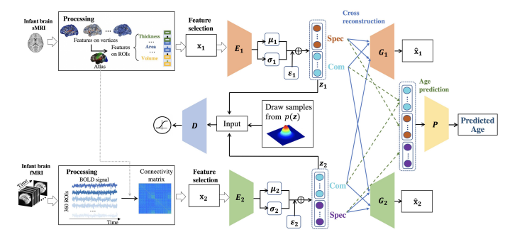
To address this issue, we develop a novel model termed as disentangled-multimodal adversarial autoencoder (DMM-AAE) for infant age prediction based on multimodal brain MRI.
Specifically, we disentangle the latent variables of autoencoder into common and specific codes to represent the shared and complementary information among modalities, respectively.
Then, crossreconstruction requirement and common-specific distance ratio loss are designed as regularizations to ensure the effectiveness and thoroughness of the disentanglement.
By arranging relatively independent autoencoders to separate the modalities and employing disentanglement under cross-reconstruction requirement to integrate them, our DMM-AAE method effectively restrains the possible interference cross modalities, while realizing effective information fusion.
Taking advantage of the latent variable disentanglement, a new strategy is further proposed and embedded into DMM-AAE to address the issue of incompleteness of the multimodal neuroimages, which can also be used as an independent algorithm for missing modality imputation.
By taking six types of cortical morphometric features from sMRI and brain functional connectivity from fMRI as predictors, the superiority of the proposed DMMAAE is validated on infant age (35 to 848 days after birth) prediction using incomplete multimodal neuroimages.
The mean absolute error of the prediction based on DMMAAE reaches 37.6 days, outperforming state-of-the-art methods. Generally, our proposed DMM-AAE can serve as a promising model for prediction with multimodal data.

논문에서 제안하는 DMM-AEE (disentangled-multimodal adversarial autoencoder)은 서로 다른 2개의 modality (multi-modality)를 합성하는 AAE (Adversarial Autoencoders)모델이다.
논문에서 저자가 제안하는 Model은 각각의 Modality의 Encoder에서 Complementary Information을 가지는 Latent representation뿐만 아니라 Consensus Information을 가지는 Latent representation도 학습할 수 있는 Model을 제시한다.

Introduction

However, considering the relatively low spatial resolution and high noise level of fMRI, as well as the immature and dramatically changing functional connectivity derived from it, it is infeasible or ineffective to directly fuse fMRI and sMRI data by conventional multimodal fusion strategies [10],[16]. These strategies may even reduce the accuracy of only using features derived from sMRI, which have been verified as robust biomarkers for predicting infant age [17].
However, traditional autoencoders always mix shared information and complementary information from different modalities into a single latent variable, where the information from one modality may act as the noise obstructing the reconstruction of the other. Thus, the main challenge for an effective fusion of sMRI and fMRI data is to reduce the negative impact from one modality to the other in the fusion process.
we designed a cross-reconstruction requirement and a common-specific distance ratio as regularizations to guarantee the effectiveness of the disentanglement and the integrity of the combined information.
we proposed an imputation algorithm for missing modality data by employing the shared information and specific information represented by the disentangled latent variable.

Multi-modality를 사용하는 과정에서의 어려움과 그를 해결하기 위한 해결책으로서 자신들의 model을 제안한다.
먼저, 논문저자들이 Multi-modality의 문제점으로 삼은 것은 크게 2가지이다.

첫째, Modality의 중요도가 서로 다르다는 것 이다. 해당 논문에서 사용하는 Dataset은 sMRI와 fMRI이다. 현재 논문에서 수행하는 Task는 fMRI는 noisy가 크며 performance가 낮은 것을 알 수 있다. 이러한 modality는 다른 modality와 함께 사용할 때 Performance를 낮추게 된다.
이러한 문제점을 해결하기 위하여 각각의 modality의 개인적인 정보인 complementary information과 공통적인 정보인 consensus information을 뽑을 수 있는 model을 제안한다. 즉, 상대적으로 도움이 안되는 fMRI에서 sMRI와 공통적인 정보를 사용함으로 인하여 classification에 도움을 줄 수 있는 feature를 선택하는데 도움을 받을 수 있다.

둘째, Inocomplement Data이다. 많은 Bio Data는 각각의 modality별로 공통적인 subject는 적다. 따라서 해당 저자는 자신들이 제안하는 model을 활용하게 되면 missing modality의 value를 estimation할 수 있다.

Dataset

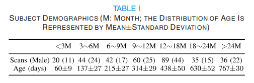
• Goal: Age prediction
• Number of dataset: 178
• Modality:
  • T1-MRI
    • Number of sample: 326
    • Number of feature: 64,620 (360 [ROI] X 6 types of features [local gyrification index (LGI), average convexity, mean curvature, corticical thickness, surface area, cortical volume])
  • fMRI
    • Number of sample: 171
    • Number of feature: 360 X 360 (Pearson’s Correlation)

Methods

Notation

• \(N\): Number of samples
• \(x_{1n} \in \mathbb{R}^{m1}\): 1-st modality n-th input (after feature selection)
• \(x_{2n} \in \mathbb{R}^{m2}\): 2-nd modality n-th input (after feature selection)
• \(y_{1n}\): 1-st modality n-th label
• \(y_{2n}\): 2-nd modality n-th label
• \(E_i\): i-th encoder
• \(E_i(x_{in}) = z_{in}, i=1,2, n=1,2,\ldots,N\): i-th modality n-th latent variable
• \(G_i\): i-th decoder
• \(Com(z_i)\): common code representing the shared information amongst modalities
• \(Spec(z_i)\): specific code representing the complementary information that differentiates one modality from the other
• \(P\): Classifier
• \(D\): Shared Discriminator (For Adversarial Autoencoder)

The framework of the proposed method: DMM-AAE

Feature Selection
현재 논문에서 사용하는 2개의 modality는 모두 sample에 비하여 feature가 많다. 따라서 Feature Selection을 Random Forest로서 각각 \(m1, m2\)개 만큼 Selection을 하였다. 각 fature의 정확한 개수는 적혀있지 않다.

Cross Reconstruction
해당 논문은 다음과 같이 reconstruction의 목적을 정하였다. 먼저, Latent Vairable (\(z_i\))는 complementary information을 가지고 있는 \(Com(z_i)\)와 \(Spec(z_i)\)로 구성되어있다.
이 중, \(Com(z_i)\)는 modality간에 공유되는 정보이므로, 다른 modality또한 reconstruction할 수 있도록 정보를 제공하여야 한다.
또한, \(Spec(z_i)\)는 modality만의 특수한 정보이므로, \(Com(z_i)\)와 함께 reconstruction을 잘 수행할 수 있도록 강조하는 역할을 할 수 있다.

Age Prediction (Classification)

$$M(x_1, x_2) = (Common_{1,2}, Spec(E_1(x_1)), Spec(E_2(x_2)))$$

$$Common_{1,2} = \sum_{i=1}^2 w_i Com(E_i(x_i))$$

$$\hat{y} = P(M(x_1, x_2))$$

해당 논문에서 최종적인 classification은 위의 식대로 Common information과 Complementary Information을 모두 Input으로 사용하여 prediction한다. \(w_1, w_2\)는 각 modality의 중요도를 설정할 수 있는 hyperparameter이며, 해당 논문은 두 값을 모두 0.5로서 동일한 값으로 지정하였다.

Adversarial Loss

• \(p(z_i)\): Arbitary Prior
• \(q(z_i) = \int_{x_i} q(z_i|x_i)p_d(x_i) d x_i\): Aggreated posterior
• \(q(z_i|x_i)\): Encoding distribution
• \(p(x_i|z_i)\): Decoding distribution

위와 같이 Notation을 정리하면 기존에 알려진 AAE와 동일하게 Adversarial Loss를 아래와 같이 정의할 수 있다.

$$L_{adv} = L_{adv}^1 + L_{adv}^2, (L_{adv}^i = \text{i-th modality Adversarial Loss})$$

또한, 해당 논문은 VAE와 마찬가지로 가장 흔한 형태인 \(p(z_i) \sim N(\mu_i(x_1), \sigma_i(x_i))\)로서 Gaussian Distribution으로 정의하였다. 따라서 Backpropagation을 진행할 때 reparameterization trick을 사용하게 된다.

Common-Specific Distance Ratio Loss

$$L_{Disen} = L_{Disen}^{Com}/L_{Disen}^{Spec}$$

$$L_{Disen}^{Com} = \mathbb{E}_{x_1, x_2} \| Com(E_1(x_1)) - Com(E_2(x_2))\|_2$$

$$L_{Disen}^{Spec} = \mathbb{E}_{x_1, x_2} \| Spec(E_1(x_1)) - Spec(E_2(x_2))\|_2$$

위의 Loss를 살펴보게 되면, 각각의 Modality의 특성을 가지는 (Complementary Information) Latent Representation은 서로 다를수록, Modality의 공통의 특성을 가지는 (Consensus Information) Latent Represenation은 서로 비슷할수록 Loss가 줄어드는 것을 확인할 수 있다.

Regression Loss

$$L_{reg} = \mathbb{E}_{x_1, x_2} \| y - P(M(x_1, x_2))\|_2$$

기존의 Regression과 마찬가지로 MSE로서 Loss를 구성하였다.

Reconstruction Loss

$$L_{recon} = \sum_{i=1}^2 \sum_{j=1}^2 \mathbb{E}_{x_i p_d(x_i)} \| x_i - G_i (Com(E_j(x_j)), Sepc(E_i(x_i)))\|_2$$

위의 Loss는 Reconstruction Loss로서 많이 사용하는 MSE Loss로서 구성하였다.
Reconstruction Loss를 구성할 때 주의하여야 하는 점은 Target의 Modality와 Common Represenation의 Modality가 다른 Cross Reconstruction으로서 Loss를 구성하였다는 것 이다.

Full Objective

$$L_D = L_{adv}$$

$$L_{E_i, G_i, P} = \lambda_1 L_{reg} + \lambda_2 L_{disen} + L_{recon} + \lambda_3 L_{adv E}$$

$$\lambda_1, \lambda_2, \lambda_3: \text{trade-off parameters}, L_{advE} = \sum_{i=1}^2 \mathbb{E}_{x_1 \sum p_d(x_i)} \log(1-D(E_i(x_i)))$$

해당 논문에서 제시하는 DMM-AEE는 먼저 \(L_D\)를 활용하여 \(z\)를 통해 sampling을 할 수 있게 Update한다. 그 뒤, \(L_{E_i, G_i, P}\)를 통하여 Consensus Information과 Common Information을 Latent Representation으로 나타낼 수 있도록 Update함과 동시에 Age를 Prediciton할 수 있는 model을 제안한다.

해당 논문은 Code를 제공하고 있지 않습니다. 따라서 위의 순차적으로 update하는 과정이 한 epoch에서 이루워지는 지 혹은, \(L_D\)로서 모두 update하고 뒤의 과정을 진행하는 지는 알 수 없었습니다.

해당 논문에는 다음과 같이 적혀 있습니다.

DMMAAE first updates its discriminative network \(D\) to tell apart the true samples (generated using the prior) from the generated samples (the latent vector computed by the encoder \(E_i\)) with \(L_D\), and then updates its encoder \(E_i\) , decoder \(G_i\) , and predictor \(P\) with \(L_{E_i, G_i, P}, i = 1, 2.\)

위의 수식과 설명을 봤을때의 개인적인 생각으로는 먼저 D를 학습함과 동시에 z를 통하여 sampling을 할 수 있는 model을 먼저 구축한다 (모든 epoch를 다 돌려서 loss가 최소화 되게 학습한다). 그 뒤, 학습된 model을 가지고 뒤의 step으로서 학습하는 two-step구조로서 학습한다고 생각된다. 두번째 step에서는 더이상 noise에서 sampling을 고려할 필요하 없기 때문에 \(L_{adv E}\)를 사용하는 것 같다.

참조. AAE vs VAE
해당 논문에서 VAE를 사용하지 않고, AAE를 사용한 것에 대하여 다음과 같이 언급하고 있다.

Except AAE, VAE is also capable of imposing prior distribution on the latent variable. VAE uses KL divergence penalty to enforce the aggregated posterior of the latent variable to simulate the prior distribution, while AAE uses an adversarial discriminator to do so. Compare with VAE, AAE may be superior on capturing the data manifold and imposing complicated prior distribution without exact functional form. AAE is possibly more general in various application scenarios. Thus, in our work, AAE is chosen to impose a prior distribution on the latent variable

Data Imputation for Missing Modality

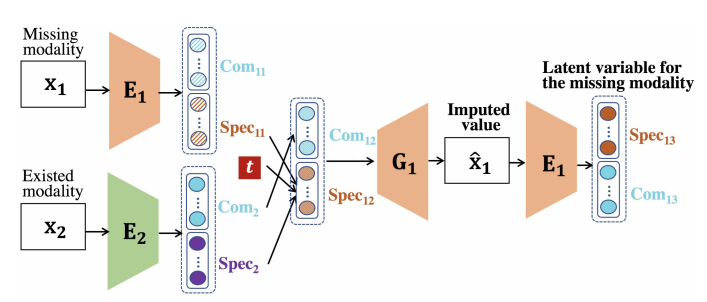
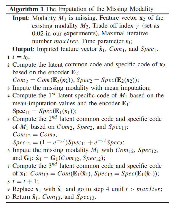
Data imputation for missing modality의 Algorithm을 살펴보면, 해당 과정은 아래와 같다.

1. \(M_1\)은 몇몇 sample이 없는 incomplement modality로서 가정하고, \(M_2\)은 모든 sample이 있는 modality로서 가정한다.
2. \(Com (E_1(x_1))\)는 \(L_{Disen}^{Com}\)을 통해 \(Com (E_2(x_2))\)와 비슷해지므로 같은 값으로서 사용한다. 또한, \(L_{recon}\)에서 Common값은 다른 modality로서 학습하므로, Generation에서도 \(Com (E_2(x_2))\)의 값을 그대로 사용한다.
3. \(Spec_{12} = (1-e^{-\gamma t})Spec_{11} + e^{-\gamma t} Spec_2, Spec_{11} = \text{mean-imputation values}\)로서 처음에는 modality2로서 학습하나, epoch가 지날 수록 Modality 1의 평균값으로 대치한다.

Result

Age Classification

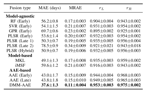
기존의 다른 Model에 비하여 Error가 낮은 것을 알 수 있다. 또한, Encoder에 Base Model이 되는 AAE에 비하여 더 좋은 것을 알 수 있다. Missin Modality의 경우에는 “Zero Imputation”으로서 0값으로 채워 수행하였다.

Comparison Between Multi-Modality and Uni-Modality

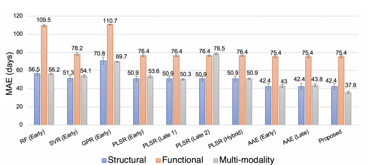
대부분의 다른 Model은 Multi-modality로서 사용하게 되면, 성능이 좋지 않은 Functional MRI때문에 성능이 하향되는 것을 알 수 있다. 하지만, DMM-AEE는 성능이 더 좋아지는 것을 확인할 수 있다.

Comparison Related to Imputing the Missing Modality

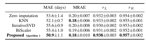
위의 Performance는 다른 Method와 Missing Modality의 값을 여러 방법으로 대체해서 performance를 비교한 값 이다. Model은 PLSR (Early)를 사용하였다. 모든 Performance에서 최고 성능을 보인 것을 알 수 있다.

Importance Analysis of the Features

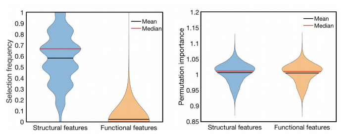
• Selection frequency는 Random Forest Model을 OOB(Out-of-Bag)으로서 feature importance를 측정한 방법이다.
• Permutation importance는 DMM-AEE Model을 permutation importance로서 \(PI(f) = \text{Error}^{orig}/\text{Error}^{perm}\)으로서 측정하였다.

해당 결과를 살펴보게 되면, 단순한 random forest 방법으로서는 classification에 도움을 주는 modality에서만 feature를 선택하는 반면, DMM-AEE는 사용한 modality에서 동일하게 important feature를 선택할 수 있는것을 알 수 있다.