Paper27. Addressing Failure Prediction by Learning Model Confidence

Addressing Failure Prediction by Learning Model Confidence

• Paper: Addressing Failure Prediction by Learning Model Confidence
• Code: valeoai Github

Abstract

Assessing reliably the confidence of a deep neural network and predicting its failures is of primary importance for the practical deployment of these models. In this paper, we propose a new target criterion for model confidence, corresponding to the True Class Probability (TCP). We show how using the TCP is more suited than relying on the classic Maximum Class Probability (MCP). We provide in addition theoretical guarantees for TCP in the context of failure prediction. Since the true class is by essence unknown at test time, we propose to learn TCP criterion on the training set, introducing a specific learning scheme adapted to this context. Extensive experiments are conducted for validating the relevance of the proposed approach. We study various network architectures, small and large scale datasets for image classification and semantic segmentation. We show that our approach consistently outperforms several strong methods, from MCP to Bayesian uncertainty, as well as recent approaches specifically designed for failure prediction.

해당 논문에서는 많은 이전 논문들에서 Classification or Segmentation 등 많은 Task에서 사용되는 Softmax로서 Confidence를 추정하는 방법에 대한 문제점을 제시한다. 이러한 문제점을 해결하기 위한 방법인 TCP (True Class Probability)로서 Confidence를 추정하고, 이를 활용하여 Model의 Performance를 높이는 방법을 제안한다.

Introduction

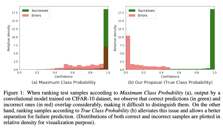
Despite their growing success, safety remains a great concern when it comes to implement these models in real-world conditions [1, 19] Another important issue related to MCP, which we specifically address in this work, relates to ranking of confidence scores: this ranking is unreliable for the task of failure prediction [41, 20]. As illustrated in Figure 1(a) for a small convolutional network trained on CIFAR-10 dataset, MCP confidence values for erroneous and correct predictions overlap. It is worth mentioning that this problem comes from the fact that MCP leads by design to high confidence values, even for erroneous ones, since the largest softmax output is used. On the other hand, the probability of the model with respect to the true class naturally reflects a better behaved model confidence, as illustrated in Figure 1(b). This leads to errors’ confidence distributions shifted to smaller values, while correct predictions are still associated with high values, allowing a much better separability between these two types of prediction.

이전의 많은 A.I. Model의 Output은 Softmax를 마지막 출력 Output의 Layer로서 사용하여, Probability를 뽑을 수 있게 설계하였다. 하지만, 이러한 Softmax의 사용은 단순히 Probability가 상대적으로 높은것을 Output으로 뽑기 때문에, Error Prediction에 대하여도 높은 Confidence를 가지게 한다 (Figure 1(a)). 이러한 문제점을 해결하기 위하여 해당 논문에서 제시하는 방법은 Figure 1(b)와 같이 정확히 Prediction한 부분에 대해서는 높은 Confidence를 유지하면서, Error로서 예측한 Sample에 대해서는 낮은 Confidence를 가지도록 Model을 학습하는 방법을 제시한다.

Notation

• \(x_i \in \mathbb{R}^d\): d-dimensional feature
• \(y_i^* \in \mathbb{Y} = \{1, \ldots, K\}\): true class
• \(N\): number of samples.
• \(D = \{ (x_i,y_i^*)\}_{i=1}^N\): training samples (i.i.d)
• \(P(Y|w,x)\): probabilistic predictive distribution by computing the softmax output for each class k
• \(\hat{y} = \text{argmax}_{y \in \mathbb{Y}} P(Y=k|w,x)\): class predicted by the model

위와 같이 Notation을 정의하였을 때, 우리는 기존에 사용하던 Softmax의 Lossfunction을 아래와 같이 적을 수 있다. (NLL Loss)

$$L_{CE}(w;D) = - \frac{1}{N} \sum_{i=1}^N y_i^* \text{log}(Y=y_i^*|w,x_i)$$

Confidence criterion for failure prediction

해당 논문에서 먼저, Softmax의 Output을 Confidence로서 사용하게 되면 아래와 같은 식으로서 표현할 수 있게 된다.

$$\text{Maximum Class Probability}: \text{MCP}(x) = \text{max}_{k \in \mathbb{Y}}P(Y=k|w,x) = P(Y=\hat{y}|w,x)$$

Softmax는 Class개수만큼의 Probability중에서 값이 큰 것을 Prediction으로서 사용하는 방법이기 때문에, Error prediction에 대해서도 큰 Confidence값을 가지게 된다.

위와 같은 문제점을 해결하기 위하여 해당 논문에서는 실제 Label에 대한 Confidence를 추가적으로 사용하게 된다. 이러한 값은 “True Class Probability”라고 정의하면, 아래와 같이 정의하게 된다.

$$\text{True Class Probability}: \text{TCP}(x, y^*) = P(Y=y^*|w,x)$$

• \(\text{TCP}(x, y^*) > 1/2 \rightarrow \hat{y}=y^*\), i.e. the example is properly classified by the model,
• \(\text{TCP}(x, y^*) < 1/K \rightarrow \hat{y} \neq y^*\), i.e. the example is wrongly classified by the model.

위와 같은 TCP에서 조건에 따라 다른 값을 가지는 것은 “Appendix 1. Proof of TCP theoretical guarantees”에 설명되어 있다. 또한, TCP의 문제점으로서 [1/K, 1/2]에서는 값을 정의할 수가 없다. 이러한 문제점에 대하여 실제 Dataset과 Model을 학습하였을때, 위의 사잇값의 Probability는 거의 존재하지 않기 때문에 따로 정의하지 않았다고 적혀있다. 이는 최근 A.I. Model들이 Overfitting되는 경향 때문이며, 이는 “Appendix 2. Calibration”에 적혀있다.

해당 논문은 실제 많이 사용하는 MCP와 TCP를 사용하여 normlaization variant of the TCP를 아래와 같은 식으로서 표현하였다.

$$\text{The ratio between TCP and MCP}: \text{TCP}^r(x, y^*) = \frac{P(Y=y^*|w,x)}{P(Y=\hat{y}|w,x)}$$

Appendix 1. Proof of TCP theoretical guarantees

Case 1. \(\text{TCP}(x, y^*) > 1/2 \rightarrow \hat{y}=y^*\)

$$\text{TCP}(x, y^*) = P(Y=y^*|w,x) > \frac{1}{2}$$

$$\Leftrightarrow 1 - \sum_{k \in \mathbb{Y}, k \neq y^*} P(Y=k|w,x) > \frac{1}{2}$$

$$\Leftrightarrow \sum_{k \in \mathbb{Y}, k \neq y^*} P(Y=k|w,x) < \frac{1}{2}$$

$$\Leftrightarrow P(Y=k|w,x) < \frac{1}{2} < P(Y=y^*|w,x), \forall k \neq y^*$$

Case 2. \(\text{TCP}(x, y^*) < 1/K \rightarrow \hat{y} \neq y^*\)

$$P(Y=y^*|w,x) < \frac{1}{K}(1)$$

$$\Leftrightarrow 1 - \sum_{k \in \mathbb{Y}, k \neq y^*} P(Y=k|w,x) < \frac{1}{K}$$

$$\Leftrightarrow \sum_{k \in \mathbb{Y}, k \neq y^*} P(Y=k|w,x) > \frac{K-1}{K}(2)$$

만약, \(\hat{y}=y^*\)로서 model이 예측을 잘 했다면, \(\forall k \neq y^*, P(Y=y^*|w,x) \ge P(Y=k|w,x)\)의 두 조건을 만족하는 것을 알 수 있다. 해당 조건과 (1) 식을 같이 사용하게 되면 다음과 같이 식을 쓸 수 있다.

$$\sum_{k \in \mathbb{Y}, k \neq y^*} P(Y=k|w,x) \le (K-1)P(Y=y^*|w,x) \le \frac{K-1}{K}(3)$$

(2)와 (3)의 조건을 합치면 아래의 식과 같으면, 이는 모순되는 것을 알 수 있다.

$$\frac{K-1}{K} < (K-1)P(Y=y^*|w,x) \le \frac{K-1}{K}$$

즉, \(\text{TCP}(x, y^*) < 1/K\)의 경우에는 항상 \(\hat{y}=y^*\)일 수 없으므로, \(\hat{y} \neq y^*\)이다.

Appendix 2. Calibration
해당 Section은 Deep Play:티스토리의 내용을 그대로 가져왔습니다.

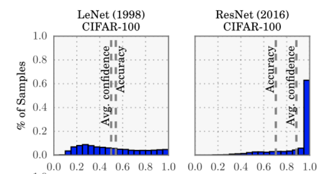
Calibration 이란 모형의 출력값이 실제 confidence를 반영하도록 만드는 것입니다. 예를 들어, X 의 Y1 에 대한 모형의 출력이 0.8이 나왔을 때, 80 % 확률로 Y1 일 것라는 의미를 갖도록 만드는 것입니다. 일반적으로 현대 딥러닝은 overconfident 합니다. 아래 그림은 1998 년 제시된 LeNet 과 2016년 제시된 ResNet (110 layer) 의 calibration 을 비교한 그림입니다. LeNet 의 경우 모형의 출력이 0~1 사이에 균일하게 분포되어있는 것을 볼 수 있지만, ResNet 의 경우 1 근처에 집중되어 있다는 것을 볼 수 있습니다. 그 결과로 아래 그림을 보면, ResNet 의 경우, confidence 와 accuracy가 많이 어긋난다는 것을 볼 수 있습니다.

Learning TCP confidence with deep neural networks

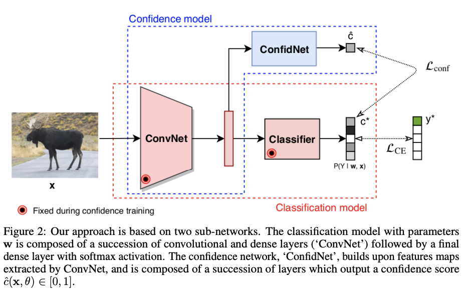
TCP를 사용하기 위한 제일 큰 문제점은 Test과정에서 실제 Label에 대한 정보는 사용할 수 없다는 것 이다. 따라서 해당 논문은 Label에 대한 Probability를 뽑아내기 위하여 위의 Figure와 같이 “Confidence network”를 추가적으로 사용하였다.

Confidence network design.
위에서 추가한 Confidence net은 2D feature map을 Input으로 사용하여 \(P(Y=y^*|w,x)\)를 예측하도록 학습된다. 따라서 Output단은 Sigmoid를 사용하게 되었다.

Loss Function.
Loss function은 Regression의 문제와 마찬가지로 MSE Loss를 사용하였다.

$$Loss_{conf}(\theta;D) = \frac{1}{N} \sum_{i=1}^N (\hat{c}(x_i, \theta) - c^*(x_i, y_i))^2, \theta \text{ is parameter of confidence network}$$

-\(\theta\): parameter of confidence network
-\(c^*(x_i, y_i) = P(Y=y^*|w,x)\): parameter of confidence network
-\(\hat{c}(x_i, \theta) \in [0,1]\): output of confidence network

Learning scheme.

1. 기존과 동일하게 Feture Extractor(ConvNet)과 Classifier를 학습
2. Fearture Extractor와 Classifier를 고정하고, ConfidNet을 학습.
3. In a next step, we can then fine-tune the ConvNet encoder. However, as model M has to remain fixed to compute similar classification predictions. -> 논문에서는 추가적인 Fine-Tuning이 별로 효과가 없다라고 나와있습니다. 또한, Code상이나 실제 논문에서 어떻게 Fine-Tuning하였는지는 적혀있지 않습니다.

개인적으로는, ConfidenceNet을 통하여 추가적인 ConvNet or Encoder부분을 학습해야지 의미있지 않나 생각하였습니다. 하지만, 현재 논문의 Goal은 Binary로서 맞췄는지 틀렸는지가 가낭 중요한 문제 입니다. 따라서, 추가적인 TCP를 사용하여 OOD sample을 제거하는 것이 목표이므로 이러한 추가적인 과정을 필요 없다고 생각됩니다.

최종적인 Prediction은 \(P(Y=k|w,x)\)와 Confidence Output인 \(\hat{c}(x_i, \theta)\)을 활용하여 예측합니다. (하지만, Prediction은 중요하지 않은 Metric으로서 평가하게 됩니다.)

해당 논문에서 계속하여 의문이 든 점은 Prediction의 결과에 대하여 다른 Class로서 어떻게 예측하냐 였다. 즉, \(\text{TCP}(x,y^*) < 1?K\)인 경우이다. 이러한 문제에 대하여, 해당 논문은 어떻게 Prediction한다라고 나와있지 않고, 해당 Class가 아니다로서만 예측가능 할 것 이다. 또한 이러한 Prediction에서 사용할 수 있는 Metric들은 Experimemt에서 사용하였다. (Appendix 4. Metric example)참조.

Pytorch Code

Model Code는 MLP, Small convolutional network, VGG-16, SegNet 중 MLP기준으로 설명합니다.

MLP (Feature Extractor + Classifier)

class MLP(AbstractModel):
    def __init__(self, config_args, device):
        super().__init__(config_args, device)
        self.dropout = config_args["model"]["is_dropout"]
        self.fc1 = nn.Linear(
            config_args["data"]["input_size"][0] * config_args["data"]["input_size"][1],
            config_args["model"]["hidden_size"],
        )
        self.fc2 = nn.Linear(
            config_args["model"]["hidden_size"], config_args["data"]["num_classes"]
        )
        self.fc_dropout = nn.Dropout(0.3)

    def forward(self, x):
        out = x.view(-1, self.fc1.in_features)
        out = F.relu(self.fc1(out))
        if self.dropout:
            if self.mc_dropout:
                out = F.dropout(out, 0.3, training=self.training)
            else:
                out = self.fc_dropout(out)
        out = self.fc2(out)
        return 

Feature Extractor

class MLPExtractor(AbstractModel):
    def __init__(self, config_args, device):
        super().__init__(config_args, device)
        self.dropout = config_args["model"]["is_dropout"]
        self.fc1 = nn.Linear(
            config_args["data"]["input_size"][0] * config_args["data"]["input_size"][1],
            config_args["model"]["hidden_size"],
        )

    def forward(self, x):
        out = x.view(-1, self.fc1.in_features)
        if self.dropout:
            out = F.dropout(out, 0.3, training=self.training)
        out = F.relu(self.fc1(out))
        return out

ConfidNet

class MLPSelfConfid(AbstractModel):
    def __init__(self, config_args, device):
        super().__init__(config_args, device)
        self.dropout = config_args["model"]["is_dropout"]
        self.fc1 = nn.Linear(
            config_args["data"]["input_size"][0] * config_args["data"]["input_size"][1],
            config_args["model"]["hidden_size"],
        )
        self.fc2 = nn.Linear(
            config_args["model"]["hidden_size"], config_args["data"]["num_classes"]
        )
        self.fc_dropout = nn.Dropout(0.3)

        self.uncertainty1 = nn.Linear(config_args["model"]["hidden_size"], 400)
        self.uncertainty2 = nn.Linear(400, 400)
        self.uncertainty3 = nn.Linear(400, 400)
        self.uncertainty4 = nn.Linear(400, 400)
        self.uncertainty5 = nn.Linear(400, 1)

    def forward(self, x):
        out = x.view(-1, self.fc1.in_features)
        out = F.relu(self.fc1(out))
        if self.dropout:
            if self.mc_dropout:
                out = F.dropout(out, 0.3, training=self.training)
            else:
                out = self.fc_dropout(out)

        uncertainty = F.relu(self.uncertainty1(out))
        uncertainty = F.relu(self.uncertainty2(uncertainty))
        uncertainty = F.relu(self.uncertainty3(uncertainty))
        uncertainty = F.relu(self.uncertainty4(uncertainty))
        uncertainty = self.uncertainty5(uncertainty)

        pred = self.fc2(out)
        return pred, uncertainty

Experiments

Experimental setup

• Dataset:
  • MNIST
  • SVHN
  • CIFAR-10
  • CIFAR-100
  • CamVid
• Network architectures:
  • MNIST: MLP
  • MNIST, SVHN: Small convolutional network
  • CIFAR: VGG-16
  • CamVid: SegNet
• Evaluation metrics: AUPR-Error, AUPR-Success, FPR at 95%-TPR, AUROC
  • AUCPR-Success는 Label 맞춘 것을 1, 틀린 것은 0으로서 새로운 Label로 정의하고 Probability와 AUPR을 구하였다.
  • AUCPR-Error는 Label을 틀린 것을 1, 맞은 것은 0으로서 새로운 Label로 정의하고 -1*Probability와 AUPR을 구하였다.

즉, 모든 Metric에서 맞은 것에 대한 Confidence가 높으며, 틀린 것에 대한 Confidence가 낮은 경우 performance가 높도록 Experiment Metric을 구성하였다.

import torch
import torch.nn.functional as F

import numpy as np
from sklearn.metrics import average_precision_score, roc_auc_score, auc

# Model Prediction
output = torch.tensor([[0.1, 0.2, 0.7], 
                       [0.2, 0.4, 0.7], 
                       [0.7, 0.1, 0.2], 
                       [0.1, 0.8, 0.3], 
                       [0.2, 0.2, 0.4]])

target = torch.tensor([2, 2, 1, 1, 0])
confidence, pred = F.softmax(output, dim=1).max(dim=1, keepdim=True)

# Value Update
accurate, errors, proba_pred = [], [], []
accuracy = 0

accurate.extend(pred.eq(target.view_as(pred)).detach().numpy())
accuracy += pred.eq(target.view_as(pred)).sum().item()
errors.extend((pred != target.view_as(pred)).to("cpu").numpy())
proba_pred.extend(confidence.detach().numpy())

# Calculate Metrics
accurate = np.reshape(accurate, newshape=(len(accurate), -1)).flatten()
errors = np.reshape(errors, newshape=(len(errors), -1)).flatten()
proba_pred = np.reshape(proba_pred, newshape=(len(proba_pred), -1)).flatten()

auc_score = roc_auc_score(accurate, proba_pred)
ap_success = average_precision_score(accurate, proba_pred)
ap_errors = average_precision_score(errors, -proba_pred)

print('Case 1.')
print('Target: ', target)
print('Prediction: ', pred.squeeze())
print('Confidence: ', confidence.squeeze())
print('AUPR-Success: ', ap_success)
print('AUPR-Error: ', ap_errors)

# Model Prediction
output = torch.tensor([[0.1, 0.2, 0.7], 
                       [0.2, 0.4, 0.7], 
                       [0.9, 0.1, 0.2], 
                       [0.1, 0.8, 0.3], 
                       [0.2, 0.2, 0.9]])

target = torch.tensor([2, 2, 1, 1, 0])
confidence, pred = F.softmax(output, dim=1).max(dim=1, keepdim=True)

# Value Update
accurate, errors, proba_pred = [], [], []
accuracy = 0

accurate.extend(pred.eq(target.view_as(pred)).detach().numpy())
accuracy += pred.eq(target.view_as(pred)).sum().item()
errors.extend((pred != target.view_as(pred)).to("cpu").numpy())
proba_pred.extend(confidence.detach().numpy())

# Calculate Metrics
accurate = np.reshape(accurate, newshape=(len(accurate), -1)).flatten()
errors = np.reshape(errors, newshape=(len(errors), -1)).flatten()
proba_pred = np.reshape(proba_pred, newshape=(len(proba_pred), -1)).flatten()

auc_score = roc_auc_score(accurate, proba_pred)
ap_success = average_precision_score(accurate, proba_pred)
ap_errors = average_precision_score(errors, -proba_pred)

print('Case 2.')
print('Target: ', target)
print('Prediction: ', pred.squeeze())
print('Confidence: ', confidence.squeeze())
print('AUPR-Success: ', ap_success)
print('AUPR-Error: ', ap_errors)

Case 1.
Target:  tensor([2, 2, 1, 1, 0])
Prediction:  tensor([2, 2, 0, 1, 2])
Confidence:  tensor([0.4640, 0.4260, 0.4640, 0.4755, 0.3792])
AUPR-Success:  0.8055555555555556
AUPR-Error:  0.75
Case 2.
Target:  tensor([2, 2, 1, 1, 0])
Prediction:  tensor([2, 2, 0, 1, 2])
Confidence:  tensor([0.4640, 0.4260, 0.5139, 0.4755, 0.5017])
AUPR-Success:  0.4777777777777778
AUPR-Error:  0.325

Experiments

Experimental setup

• Dataset:
  • MNIST
  • SVHN
  • CIFAR-10
  • CIFAR-100
  • CamVid
• Network architectures:
  • MNIST: MLP
  • MNIST, SVHN: Small convolutional network
  • CIFAR: VGG-16
  • CamVid: SegNet
• Evaluation metrics: AUPR-Error, AUPR-Success, FPR at 95%-TPR, AUROC

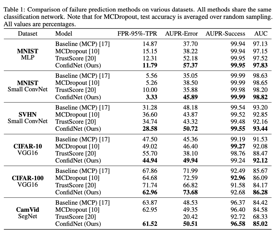
Comparative results on failure prediction.

Conclustion

해당 논문은 TCP라는 Softmax와 다르게 Prediction이 아닌 실제 Label에 대한 Confidence를 추정 할 수 있는 새로운 방법을 제시하고, 이를 사용할 수 있는 Confident-net을 제안한다. 해당 방법으로 인하여 논문은 OOD sample에 대하여 Detection을 할 수 있었다. 또한, 해당 논문은 많은 Model에서 추가적으로 사용가능한 방법이기 때문에 Genral하고, 손 쉽게 성능을 올릴 수 있는 방법이다.