Paper26. Cooperative Learning for Multi-view Analysis

Cooperative Learning for Multi-view Analysis

출처: Cooperative Learning for Multi-view Analysis
코드: dingdaisy GitHub

Abstract

We propose a new method for supervised learning with multiple sets of features (“views”). The multi-view problem is especially important in biology and medicine, where “-omics” data such as genomics, proteomics and radiomics are measured on a common set of samples. Cooperative learning combines the usual squared error loss of predictions with an “agreement” penalty to encourage the predictions from different data views to agree. By varying the weight of the agreement penalty, we get a continuum of solutions that include the well-known early and late fusion approaches. Cooperative learning chooses the degree of agreement (or fusion) in an adaptive manner, using a validation set or cross-validation to estimate test set prediction error. One version of our fitting procedure is modular, where one can choose different fitting mechanisms (e.g. lasso, random forests, boosting, neural networks) appropriate for different data views. In the setting of cooperative regularized linear regression, the method combines the lasso penalty with the agreement penalty, yielding feature sparsity. The method can be especially powerful when the different data views share some underlying relationship in their signals that can be exploited to boost the signals. We show that cooperative learning achieves higher predictive accuracy on simulated data and real multiomics examples of labor onset prediction and breast ductal carcinoma in situ and invasive breast cancer classification. Leveraging aligned signals and allowing flexible fitting mechanisms for different modalities, cooperative learning offers a powerful approach to multiomics data fusion.

제안하는 Model은 Multi-omics data fusion에 있어서 different data views (Multi-omics data)간의 squared error (agreement penalty를 포함한)를 사용하여 classification의 결과를 향상시키는 방법을 제안한다. 주요한 점은 “flexible fitting mechanisms for different modalities”를 보여주기 위하여 여러 상황에서 효과적인 방법이라는 것을 보여준다.

Introduction

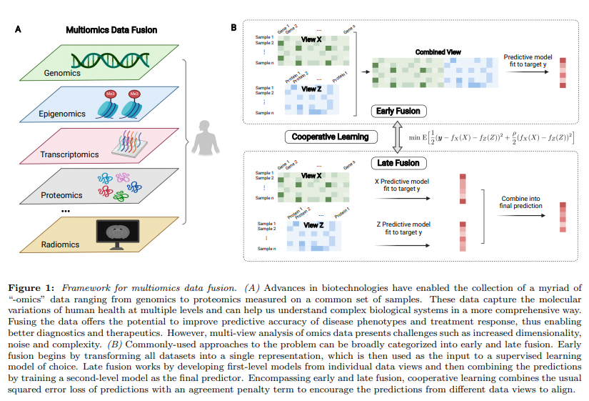
Multi-omics를 사용하는 가장 큰 이유는 2가지로서 (1) “Integrating heterogeneous features on a common set of observations provides a unique opportunity to gain a comprehensive understanding of an outcome of interest.”, (2) “It offers the potential for making discoveries that are hidden in data analyses of a single modality and achieving more accurate predictions of the outcome”이다.

Multi-views를 합성하는 방법은 전통적으로 Early Fusion과 Late Fusion이 존재한다 (Figure B). Early Fusion으로서는 간단하게 서로다른 Modality를 concat하여 하나의 Modality처럼 사용하여, 많은 model에서 사용할 수 있다는 장점이 있지만 각 modality간의 relationship을 고려할 수 없다는 단점이 있다. Late Fusion이나 Integration methods은 각각의 modality의 정보를 먼저 구축한 뒤, final prediction에 결합하는 방법이다. Late Fusion으로서는 각 Modality의 complementary information을 활용할 수 있다는 장점이 있다.

해당 논문에서는 “squared error loss of predictions with an “agreement” penalty”를 사용하여 multi-view data를 융합하는 새로운 방법 (cooperative learning)을 제안한다. 특히 제안하는 방법은 “the different data views share some underlying relationship in their signals that can be exploited to boost the signals.” 에서 강점을 보인다고 설명하고 있다. 개인적으로는 multi-omics간의 relationship이 있다고 가정하고 classificaiton을 수행하는 경우가 대부분이므로 bio domain에서 장점을 보여주는 model인 것을 알 수 있다.

Cooperative learning

Notation

• \(X \in \mathbb{R}^{n \times p_x}\): Modality 1
• \(Z \in \mathbb{R}^{n \times p_z}\): Modality 2
• \(y \in \mathbb{R}^{n}\): Label
• \(f(\cdot)\): DNN
• \(\rho \text{ s.t. }\rho \ge 0\): Hyperparameters
• \(\theta_x\): Parameters of linear regression for modality 1
• \(\theta_z\): Parameters of linear regression for modality 2
• \(\rho \text{ s.t. }\rho \ge 0\): Hyperparameters
• \(P\): Penalty (e.g., L1, L2)
• \(X_i \in \mathbb{R}^{n \times p_i}\): m-th Modality
• \(f_{X_m}(\cdot)\): m-th DNN
• \(\theta_i\): Parameters of m-th modality

Cooperative learning with two data views
DNN을 사용하는 경우 cooperative learning의 loss function은 아래와 같다.

$$\text{min} E[\frac{1}{2}(y- f_X(X) - f_Z(Z))^2 + \frac{\rho}{2}(f_X(X) - f_Z(Z))^2]$$

• \(\frac{1}{2}(y- f_X(X) - f_Z(Z))^2\): Prediction Error
• \(\frac{\rho}{2}(f_X(X) - f_Z(Z))^2\): Agreement Penalty

Agreement Penalty는 “contrastive learning”와 연관되어 있다고 한다 (뒤에 설명).
위의 Loss function은 아래의 값으로서 minimize된다.

$$f_X(X) = E[\frac{y}{1+\rho} - \frac{(1-\rho)f_Z(Z)}{1+\rho}|X]$$

$$f_Z(Z) = E[\frac{y}{1+\rho} - \frac{(1-\rho)f_X(X)}{1+\rho}|Z]$$

위의 solution을 살펴보게 되면, 하나의 prediction값이 고정되었을때, 다른 \(f(\cdot)\)을 학습할 수 있는 것을 알 수 있다. 따라서 반복적으로 각 modality의 \(f(\cdot)\)을 학습하는 것을 알 수 있다.

저자들은 위의 Loss function을 다음과 같은 2가지 경우에 대하여 나누어서 설명한다.

• \(\rho=0\): Early Fusion이다. 위의 Loss Function을 살펴보는 경우, \(f_X(X)\)와 \(f_Z(Z)\)는 일치할 필요가 없기 때문이다. 즉, abstract에서 설명한대로 각 modality간의 관계를 전혀 고려하지 않기 때문이다.
• \(\rho=1\): Late Fusion이다. \(f_X(X)\)와 \(f_Z(Z)\)가 일치할 수록 loss의 값은 작아지며, 가중치는 loss function의 first term과 동일하다. 즉, 각 modality의 dnn의 prediction값이 비슷할 수록 loss가 작아진다.

위의 cooperative learning이 반복적으로 학습하는 방식을 “one-at-a-time”이라 하며 많이 사용되는 regression, CNN, RNN기반의 model에 적용하여 설명한다.

Cooperative regularized linear regression

Regularized linear regression을 사용하는 경우 loss function은 아래와 같다.

$$J(\theta_x, \theta_z) = \frac{1}{2} \| y - X\theta_x - Z\theta_z \|^2 + \frac{\rho}{2} \| (X\theta_x - Z\theta_z) \|^2 + \lambda_x P^x(\theta_x) + \lambda_z P^z(\theta_z)$$

위의 Loss function에서 Penalty function인 \(P(\cdot)\)이 L1 Penalty로 생각하면 식은 아래와 같다.

$$J(\theta_x, \theta_z) = \frac{1}{2} \| y - X\theta_x - Z\theta_z \|^2 + \frac{\rho}{2} \| (X\theta_x - Z\theta_z) \|^2 + \lambda_x \|\theta_x\|_1 + \lambda_z \|\theta_z\|_1$$

해당 논문의 저자들인 \(\lambda_x = \lambda_z = \lambda\)로서 설정하였다. 각각의 \(\lambda\)를 다른 값으로서 지정하였을 때, 장점을 발견하지 못하였다고 한다. 각각의 \(\lambda\)를 다른 값으로 설정하는 것을 ‘adaptive cooperative learning’이라고 불리며, Appendix A.에 설명되어있다. 공통적인 \(\lambda\)를 사용하는 경우 아래와 같이 식을 단순화 할 수 있다.

$$J(\theta_x, \theta_z) = \frac{1}{2} \| y - X\theta_x - Z\theta_z \|^2 + \frac{\rho}{2} \| (X\theta_x - Z\theta_z) \|^2 + \lambda(\|\theta_x\|_1 + \|\theta_z\|_1)$$

최종적으로 Linear regression형태로 식을 만들기 위하여 아래와 같이 값을 정의하면 최종적인 식은 매우 단순화 될 수 있다.

• \(\tilde{X} = \begin{pmatrix} X & Z \\ -\sqrt{\rho}X & \sqrt{\rho}Z \end{pmatrix}\)
• \(\tilde{y} = {y \choose 0}\)
• \(\tilde{\beta} = {\theta_x \choose \theta_z}\)

$$J(\theta_x, \theta_z) = \frac{1}{2} \|\tilde{y} - \tilde{X}\tilde{\beta}\|^2 + \lambda(\|\theta_x\|_1 + \|\theta_z\|_1)$$

해당 식은 기존의 Linear regression식과 동일하다는 것을 알 수 있다. Cooperative learning with two data views과 같이 하나의 view에 대한 linear regression을 fix시키면, 다른 \(/theta\)값을 학습하여 얻을 수 있다. optimization값은 아래와 같다.

$$\hat{\theta_x} = \text{Lasso}(X, y_x^*, \lambda_x), \text{where} y_x^* = \frac{y}{1+\rho} - \frac{(1-\rho)Z\theta_z}{(1+\rho)}$$

$$\hat{\theta_z} = \text{Lasso}(Z, y_z^*, \lambda_z), \text{where} y_x^* = \frac{y}{1+\rho} - \frac{(1-\rho)X\theta_x}{(1+\rho)}$$

위와 같은 Regression 문제로서 실험한 결과는 아래와 같다.

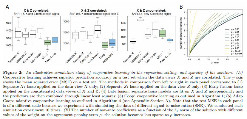
위의 Figure를 보게 되면, X, Z의 두개의 modality를 로서 fusion하여 error를 측정한 Figure이고, y-axis는 MSE이다. 해당 dataset는 SNR값이 높을수록 Error값이 작은것을 알 수 있다.

Figure A의 결과를 살펴보게 되면, 두개의 modality가 서로간의 어느정도 correlation이 있는 경우, Early fusion, Late fusion에 비하여 제안하는 cooperate learning이 효과적인 것을 알 수 있다. 이것은, SNR과 상관 없이 모두 효과적인 것을 알 수 있다.
하지만, X와 Z가 상관없는 경우에는 Cooperate learning이 효과가 없는 것을 알 수 있다. 즉, 한개의 modality만이 압도적으로 성능이 좋은 경우에는 한개의 modality만 사용하는 경우가 좋으며, 이는 Adaptive cooerate learning으로서 하나의 modality만 사용하여 X만 사용했을 때와 비슷한 성능을 내도록 하는 것 이다.

Figure B의 결과를 살펴보게 되면, agreement penalty인 \(\rho\)의 값이 클수록 Less sparse해지는 것을 알 수 있다.

Relation to early/late fusion
위의 Regression문제를 위에서 정의하였던 \(\tilde{X} = \begin{pmatrix} X & Z \\ -\sqrt{\rho}X & \sqrt{\rho}Z \end{pmatrix}\), \(\tilde{y} = {y \choose 0}\), \(\tilde{\beta} = {\theta_x \choose \theta_z}\)으로서 식을 표현하면 값은 Early Fusion과 Late Fusion으로서 생각할 수 있다. (\(l_1\) loss 생략)

$$\tilde{X}^T\tilde{X} = \begin{pmatrix} X^T X(1+\rho) & X^T Z(1-\rho) \\ Z^T X(1-\rho) & Z^T Z(1+\rho) \end{pmatrix}$$

위의 식에서 \(\rho=0\)인 경우에는 두개의 modality의 관계를 고려하는 Early fusion이라고 생각할 수 있다. 즉, \(X^TX, Z^TZ\)로서 각각의 modality의 correlation뿐만아니라, \(X^T Z, Z^T X\)로서 각각이 modality이 관계또한 생각한다는 것이다.
이와 대조적으로 \(\rho=1\)인 경우에는 각각의 modaolity는 고려하지 않는 Late Fusion인 것을 알 수 있다.

Theoretical analysis under the latent factor model

We show that the mean squared error (MSE) of the predictions from cooperative learning is a decreasing function of \(\rho\) around 0 with high probability (see details in Appendix Section D). Therefore, the agreement penalty offers an advantage in reducing MSE of the predictions under the latent factor model.

위의 문장은 이해가 되지 않았습니다… (우리는 협동 학습에서 예측의 평균 제곱 오차(MSE)가 높은 확률로 0 부근의 \(\rho\)의 감소 함수임을 보여준다(부록 섹션 D의 세부 사항 참조).)
저자들은, 제안하는 cooperative learning에서 agreement penalty가 MSE를 줄이는데 도움이 된다는 것을 Appendix D.에서 증명하였습니다.

Cooperative learning with more than two data views

이전까지의 DNN을 사용하는 경우나 regression을 사용하는 경우에는 2개의 view로서만 이루어진 결과였다. 해당 section에서는 3개 이상의 data에서도 적용한 일반적인 형태의 cooperative learning을 설명한다.

DNN을 사용하는 경우의 loss function은 다음과 같다.

$$\text{min} E[\frac{1}{2}(y- \sum_{m=1}^M f_{X_m}(X_m))^2 + \frac{\rho}{2}\sum_{m < m^{'}}(f_{X_m}(X_m) - f_{X_{m^{'}}}(X_{m^{'}}))^2]$$

$$f_{X_m}(X_m) = E[\frac{y}{1+(M-1)\rho} - \frac{(1-\rho)\sum_{m^{'} \neq m} f_{X_{m^{'}}}(X_{m^{'}})}{1+(M-1)\rho}|X_m]$$

Linear regression을 사용하는 경우는 아래와 같다.

$$J(\theta_1, \ldots, \theta_2) = \frac{1}{2} \| y - \sum_{m=1}^M X_{m}\theta_m \|^2 + \frac{\rho}{2} \sum_{m < m^{'}} \| (X_m\theta_m - X_{m^{'}}\theta_{m^{'}}) \|^2 + \sum_{m=1}^M \lambda_m \|\theta_m\|_1$$

• \(\tilde{X} = \begin{pmatrix} X_1 & X_2 & \ldots & X_{M-1} & X_M \\ -\sqrt{\rho}X_1 & \sqrt{\rho}X_2 & \ldots & 0 & 0 \\ -\sqrt{\rho}X_1 & 0 & \ldots & \sqrt{\rho}X_{M-1} & 0 \\ -\sqrt{\rho}X_1 & 0 & \ldots & 0 & \sqrt{\rho}X_M \\ 0 & -\sqrt{\rho}X_2 & \ldots & 0 & \sqrt{\rho}X_{M} \\ \ldots & \ldots & \ldots & \ldots & \ldots \\ 0 & 0 & \ldots & -\sqrt{\rho}X_{M-1} & \sqrt{\rho}X_M \end{pmatrix}\)
• \(\tilde{y} = (y \quad 0 \quad \ldots \quad 0)^T\)
• \(\tilde{\beta} = (\theta_1 \quad \theta_2 \quad \ldots \quad \theta_M)^T\)

$$\hat{\theta_m} = \text{Lasso}(X, y_m^*, \lambda_m), \text{where} y_m^* = \frac{y}{1+(M-1)\rho} - \frac{(1-\rho)\sum_{m^{'}\neq m}X_{m^{'}}\theta_{m^{'}}}{(1+(M-1)\rho)}$$

Discussion

해당 논문은 ‘agreement penalty’를 활용하여 cooperative learning을 제안하였다.
또한, 많이 사용하는 형태인 DNN과 regression뿐만 아니라, MSE를 사용하는 경우에도 해당 model 적용 방법을 제안하였다.
아쉬운 점은, 두개의 modality 중 하나의 modality만이 성능이 좋은 경우에는 성능개선이 일어나지 않는 다는 것 이다.