
Paper23. Deep learning based feature-level integration of multi-omics data for breast cancer patients survival analysis
Deep learning based feature-level integration of multi-omics data for breast cancer patients survival analysis
출처: Deep learning based feature-level integration of multi-omics data for breast cancer patients survival analysis
코드: tongli1210 GitHub
Abstract
Background: Breast cancer is the most prevalent and among the most deadly cancers in females. Patients with breast cancer have highly variable survival lengths, indicating a need to identify prognostic biomarkers for personalized diagnosis and treatment. With the development of new technologies such as next-generation sequencing, multi-omics information are becoming available for a more thorough evaluation of a patient’s condition. In this study, we aim to improve breast cancer overall survival prediction by integrating multi-omics data (e.g., gene expression, DNA methylation, miRNA expression, and copy number variations (CNVs)).
Methods: Motivated by multi-view learning, we propose a novel strategy to integrate multi-omics data for breast cancer survival prediction by applying complementary and consensus principles. The complementary principle assumes each omics data contains modality-unique information. To preserve such information, we develop a concatenation autoencoder (ConcatAE) that concatenates the hidden features learned from each modality for integration. The consensus principle assumes that the disagreements among modalities upper bound the model errors. To get rid of the noises or discrepancies among modalities, we develop a cross-modality autoencoder (CrossAE) to maximize the agreement among modalities to achieve a modality-invariant representation. We first validate the effectiveness of our proposed models on the MNIST simulated data. We then apply these models to the TCCA breast cancer multi-omics data for overall survival prediction.
Results: For breast cancer overall survival prediction, the integration of DNA methylation and miRNA expression achieves the best overall performance of 0.641 ± 0.031 with ConcatAE, and 0.63 ± 0.081 with CrossAE. Both strategies outperform baseline single-modality models using only DNA methylation (0.583 ± 0.058) or miRNA expression (0.616 ± 0.057).
Conclusions: In conclusion, we achieve improved overall survival prediction performance by utilizing either the complementary or consensus information among multi-omics data. The proposed ConcatAE and CrossAE models can inspire future deep representation-based multi-omics integration techniques. We believe these novel multiomics integration models can benefit the personalized diagnosis and treatment of breast cancer patients.
해당 논문의 주요한 Contribution은 Deep Learning기반의 새로운 Dimension Reduction기법을 통하여 Classification 성능을 올렸다는 것 이다. 해당 논문을 먼저 이해하기 전에 Multi-modality에서 많이 사용하는 complementary와 consensus라는 단어의 개념을 이해해야 한다.
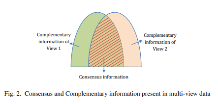
출처: A Novel Approach to Learning Consensus and Complementary Information for Multi-View Data Clustering
위의 Figure는 complementary와 consensus의 개념을 보여준다. Complementary는 각각의 modality가 가지는 특성을 의미하게 되고, Consensus는 modality와 관계없이 공통적으로 가지는 특성을 의미하게 된다.
해당 논문은 complementary를 고려하여, 각각의 modality의 특성을 사용하는 ConcatAE와 consensus를 활용하는 CrossAE의 2개의 model을 소개한다.
Methods
Dataset 1) Multi-view MNIST dataset
Model을 평가하기 위한 첫번째 Simulation Dataset은 아래와 같다.
- Training Samples: 60000
- Test Sample: 10000
- Dimension: 784(28 * 28)
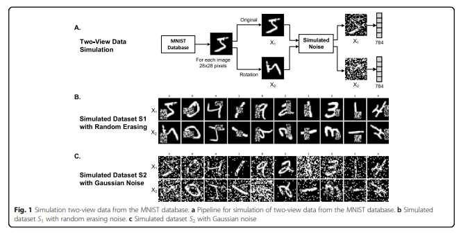
Multi-modality로 넣기 위하여 Original Image와 90도 Rotation한 Dataset을 Pair로서 사용하였다. 또한, Robust한 Model인지 확인하기 위하여, 각각의 Dataset에 Noise를 추가하였다. Noise같은 경우에는 1) Random Erasing과, Gaussian Noise를 사용하였다.
Dataset 2) TCGA-BRCA breast cancer multi-omics dataset
Model을 평가하기 위한 실제 Dataset은 다음과 같다.
- Training Sample: 60%
- Validation Sample: 15%
- Test Sample: 25%
- 5 Cross Validation
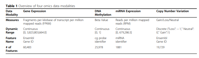
위와 같은 Dataset은 Feature가 많기 때문에, 다음과 같이 Dimension Reduction을 하여서 사용하였다.
- PCA를 이용하여 모든 Dataset의 차원을 100으로 줄였다.
- Training Sample Variance기준으로서 1000개를 사용하였다.
Single Modality Classification
Multi-modality로서 Model의 성능이 향상됬는지 확인하여 기위하여 Single-Omics Dataset에 대하여 다음과 같은 Model로서 구성하였다.
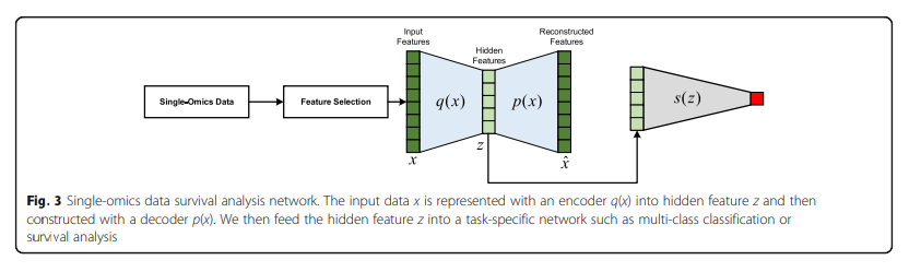
Auto Encoder로서 Dimension Reduction을 하면서 Supervised Classifier로서 Classification성능을 제공한다.
Concat AE
각각의 Modality의 Complementary를 구하기 위하여 각각의 Modality를 AutoEncoder로서 Dimension Reduction을 수행하고 Latenet Representation을 Concat하여 Classification을 수행한다.
- Feature Selection: PCA or High Variance
- Trainign Step
- 1) 각각의 Modality의 AutoEncoder학습
- 2) Classifier 학습
- 3) Classifier의 Gradient로서 각각의 Modality의 Encoder학습
Cross AE 각각의 Modality의 Consensus 구하기 위하여 각각의 Modality를 AutoEncoder로서 Dimension Reduction을 수행하고 Latenet Representation을 Element-Wise Average하여 Classification을 수행한다.
- Feature Selection: PCA or High Variance
- Trainign Step
- 1) 각각의 Modality에 맞는 AutoEncoder학습 (q1, p1, q2, p2)
- 2) Cross 하여 AutoEncoder를 학습 (q1, p2, q2, p1) => MSE Loss를 사용하였을때 Reconstrruction기준은 Decoder로서 학습한다. => 1~2의 과정에 대한 Loss는 다음과 같다. \(L_{\text{cross_recon}} = \frac{1}{N} \sum_{1}^N ((x_{1,n}-\hat{x_{12,n}})^2 + (x_{2,n}-\hat{x_{21,n}})^2)\)
- 3) Element-Wise Average하여 Consensus Latent Representation을 구함
- 3) 위의 Input으로서 Classifier를 학습
- 4) Classifier의 Gradient로서 각각의 Modality의 Encoder학습
Results
1) Multi-modality integration simulation
Simulation Data로서의 결과는 다음과 같다.
해당 결과를 살펴보게 되면 크게 2가지의 결과를 얻을 수 있다.
- Random Erasing으로서는, X1과 X2의 Information이 Random하게 사라지게 되므로, Consensus Information이 많이 줄게 되므로 각각의 Modality로서 Complementary Information을 사용하는 것이 성능이 좋다.
- Gaussian Erasing으로서는, X1과 X2의 Information이 공통적으로 줄어들게 되므로, 각각의 Modality로서 Complementary Information이 많이 줄게 되므로 Consensus Information을 사용하는 것이 성능이 좋다. (Gaussian Noise를 추가하고, 각각의 Modality는 단순히 Rotation만 수행하였으므로)
2) Multi-modality integration for breast cancer survival analysis
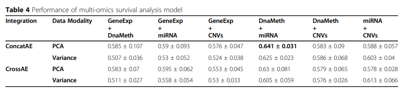
실제 Dataset을 가지고 Performance를 측정한 결과는 뚜렷하게 무엇이 좋다 라는 결과를 보여주고 있지 않다.
Discussion
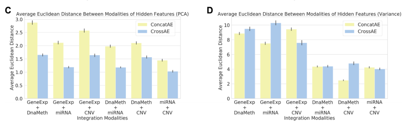
위의 그림을 살펴보게 되면 흥미로운 결과를 보여주고 있다.
먼저, PCA로서 Dimension Reduction을 하였을 경우, Variance로서 Feature Selection을 하였을 때보다, 훨씬 Similarity가 높은 것(Euclidian Distance가 작은)것을 알 수 있다.
또한, Similarity가 높을 수록 Consensus가 높으므로, Cross AE의 Euclidian Distance가 작으며, Similarity가 작을수록, Consensus는 적고 Complementary는 높으므로, Concat AE에서 Euclidian Distance가 작은 것을 알 수 있다.
Conclusion
개인적으로는 Simulation Dataset에 대한 결과는 매우 휼륭하고, Model을 설계한 대로 나오는 것을 알 수 있다. 하지만, 실제 Dataset을 적용한 Multi-Omics Classification에서는 좋은 Performance를 보여주지 않는다. Multi-Omics말고 다른 Dataset에 적용하면, 더 좋은 결과를 보여줄 Model이라고 생각한다.
Pytorch Code
해당 Model의 Cross AE와 Concat AE에 대하여 다음과 같이 간단하게 표현할 수 있다.
Encoder - \(q(\cdot)\)
1
2
3
4
5
6
7
8
9
10
11
12
13
14
15
16
17
18
19
20
21
22
23
24
25
26
27
28
class Q_net(nn.Module):
    """
    encoder: x -> z
    """
    def __init__(self, N, x_dim, z_dim, p_drop, ngpu=1):
        super(Q_net, self).__init__()
        self.ngpu = ngpu      # number of GPU
        self.x_dim = x_dim    # dimension of input features
        self.N = N            # number of neurons in hidden layers
        self.z_dim = z_dim    # dimension of hidden variables
        self.p_drop = p_drop  # probability of dropout

        self.main = nn.Sequential(
            nn.Linear(self.x_dim, self.N), #First layer, input -> N
            nn.Dropout(p=self.p_drop, inplace=True), #Dropout_1
            nn.ReLU(True), #ReLU_1
            nn.Linear(self.N, self.N), #Second layer, N -> N
            nn.Dropout(p=self.p_drop, inplace=True), #Dropout_2
            nn.ReLU(True), #ReLU_2
            nn.Linear(self.N, self.z_dim) #Gaussian code (z)
        )

    def forward(self, x):
        if isinstance(x.data, torch.cuda.FloatTensor) and self.ngpu > 1:
            z = nn.parallel.data_parallel(self.main, x, range(self.ngpu))
        else:
            z = self.main(x)
        return z
Decoder - \(p(\cdot)\)
1
2
3
4
5
6
7
8
9
10
11
12
13
14
15
16
17
18
19
20
21
22
23
24
25
26
27
28
29
class P_net(nn.Module):
    """
    Decoder: z -> x
    """
    def __init__(self, N, x_dim, z_dim, p_drop, ngpu=1):
        super(P_net, self).__init__()
        self.ngpu = ngpu      # number of GPU
        self.x_dim = x_dim    # dimension of input features
        self.N = N            # number of neurons in hidden layers
        self.z_dim = z_dim    # dimension of hidden variables
        self.p_drop = p_drop  # probability of dropout

        self.main = nn.Sequential(
            nn.Linear(self.z_dim, self.N),
            nn.Dropout(p=self.p_drop, inplace=True), #Dropout_1
            nn.ReLU(True), #ReLU_1
            nn.Linear(self.N, self.N),
            nn.Dropout(p=self.p_drop, inplace=True), #Dropout_2
            #nn.ReLU(True),
            nn.Linear(self.N, self.x_dim),
        )

    def forward(self, z):
        if isinstance(z.data, torch.cuda.FloatTensor) and self.ngpu > 1:
            x_recon = nn.parallel.data_parallel(self.main, z, range(self.ngpu))
        else:
            x_recon = self.main(z)
        return x_recon
Classifier - \(s(\cdot)\)
1
2
3
4
5
6
7
8
9
10
11
12
13
14
15
16
17
18
19
20
21
22
23
24
25
26
27
28
class C_net(nn.Module):
    """
    classificaiton network with logits (no sigmoid)
    """
    def __init__(self, N, z_dim, n_classes, p_drop, ngpu=1):
        super(C_net, self).__init__()
        self.ngpu = ngpu
        self.N = N             # number of neurons in hidden layers
        self.z_dim = z_dim     # dimension of hidden variables
        self.p_drop = p_drop   # probability of dropout
        self.n_classes = n_classes  # number of classes

        self.main = nn.Sequential(
            nn.Linear(self.z_dim, self.N),
            nn.Dropout(p=self.p_drop, inplace=True),
            nn.ReLU(True),
            nn.Linear(self.N, self.N),
            nn.Dropout(p=self.p_drop, inplace=True),
            nn.ReLU(True),
            nn.Linear(self.N, self.n_classes),
        )

    def forward(self, z):
        if isinstance(z.data, torch.cuda.FloatTensor) and self.ngpu > 1:
            decision = nn.parallel.data_parallel(self.main, z, range(self.ngpu))
        else:
            decision = self.main(z)
        return decision
Concat AE
Concat AE에서 Training 부분의 Code는 다음과 같다.
self.n_modality: Modality의 개수net_q[i]: Encodernet_p[i]: Decodernet_c: Classifier
Stage 1: train Q and P with reconstruction loss
Code에서 Stage1을 살펴보게 되면, MSE Loss로서 Reconstruction Loss를 통하여 학습하는 것을 알 수 있다.
Stage 2: train Q and C with classification loss
Classifier로 들어가는 Latent Representation은 z_combined = torch.cat(z_list, dim=1)로서 Concat하여 들어가는 것을 확인할 수 있다.
1
2
3
4
5
6
7
8
9
10
11
12
13
14
15
16
17
18
19
20
21
22
23
24
25
26
27
28
29
30
31
32
33
34
35
36
37
38
39
40
41
42
43
44
45
46
47
48
49
50
51
52
53
54
55
56
####################################################
# Stage 1: train Q and P with reconstruction loss  #
####################################################
for i in range(self.n_modality):
    net_q[i].zero_grad()
    net_p[i].zero_grad()
    for p in net_q[i].parameters():
        p.requires_grad=True
    for p in net_p[i].parameters():
        p.requires_grad=True
for p in net_c.parameters():
    p.requires_grad=False

t0 = time()
for i in range(self.n_modality):
    z_list[i] = net_q[i](X_list[i])
    X_recon_list[i] = net_p[i](z_list[i])
    loss_mse = nn.functional.mse_loss(X_recon_list[i], X_list[i]) # Mean square error
    loss_mse_list[i] = loss_mse.item()
    loss_mse.backward()
    opt_q[i].step()
    opt_p[i].step()
t_mse = time() - t0
batch_log['loss_mse'] = sum(loss_mse_list)

####################################################
# Stage 2: train Q and C with classification loss  #
####################################################
if not survival_event.sum(0): # skip the batch if all instances are negative
    batch_log['loss_survival'] = torch.Tensor([float('nan')])
    return batch_log
for i in range(self.n_modality):
    net_q[i].zero_grad()
    for p in net_q[i].parameters():
        p.requires_grad=True
    for p in net_p[i].parameters():
        p.requires_grad=False
net_c.zero_grad()
for p in net_c.parameters():
    p.requires_grad=True

t0 = time()
for i in range(self.n_modality):
    z_list[i] = net_q[i](X_list[i])
z_combined = torch.cat(z_list, dim=1)
pred = net_c(z_combined)

loss_survival = neg_par_log_likelihood(pred, survival_time, survival_event)
loss_survival.backward()
for i in range(self.n_modality):
    opt_q[i].step()
opt_c.step()
t_survival = time() - t0
c_index = CIndex(pred, survival_event, survival_time)
batch_log['loss_survival'] = loss_survival.item()
batch_log['c_index'] = c_index
Cross AE
Cross AE에서 Training 부분의 Code는 다음과 같다.
self.n_modality: Modality의 개수net_q[i]: Encodernet_p[i]: Decodernet_c: Classifier
Stage 1: train Q and P with reconstruction loss
Code에서 Stage1을 살펴보게 되면, MSE Loss로서 Reconstruction Loss를 통하여 학습하는 것을 알 수 있다.
Stage 2: train Q and P with cross reconstruction loss
각각의 다른 Modality의 Encoder와 Decoder를 MSE Loss로서 Reconstruction Loss를 통하여 학습한다. 주요한 점은 Decoder의 Modality를 기준으로서 학습하는 것을 알 수 있다.
Stage 3: train Q and C with classification loss
Classifier로 들어가는 Latent Representation은 torch.mean(torch.stack(z_list), dim=0)로서 Element-Wise Average하여 들어가는 것을 확인할 수 있다.
1
2
3
4
5
6
7
8
9
10
11
12
13
14
15
16
17
18
19
20
21
22
23
24
25
26
27
28
29
30
31
32
33
34
35
36
37
38
39
40
41
42
43
44
45
46
47
48
49
50
51
52
53
54
55
56
57
58
59
60
61
62
63
64
65
66
67
68
69
70
71
72
73
74
75
76
77
78
79
80
81
82
83
84
85
86
87
88
89
90
###################################################
# Stage 1: train Q and P with reconstruction loss #
###################################################
for i in range(self.n_modality):
    net_q[i].zero_grad()
    net_p[i].zero_grad()
    for p in net_q[i].parameters():
        p.requires_grad = True
    for p in net_p[i].parameters():
        p.requires_grad = True
for p in net_c.parameters():
    p.requires_grad = False

t0 = time()
for i in range(self.n_modality):
    z_list[i] = net_q[i](X_list[i])
    X_recon_list[i] = net_p[i](z_list[i])
    loss_mse = nn.functional.mse_loss(X_recon_list[i], X_list[i])  # Mean square error
    loss_mse_list[i] = loss_mse.item()
    loss_mse.backward()
    opt_q[i].step()
    opt_p[i].step()

t_mse = time() - t0
batch_log['loss_mse'] = sum(loss_mse_list)

#########################################################
# Stage 2: train Q and P with cross reconstruction loss #
#########################################################
for i in range(self.n_modality):
    net_q[i].zero_grad()
    net_p[i].zero_grad()
    for p in net_q[i].parameters():
        p.requires_grad = True
    for p in net_p[i].parameters():
        p.requires_grad = True
for p in net_c.parameters():
    p.requires_grad = False

t0 = time()
for i in range(self.n_modality):
    for j in range(i + 1, self.n_modality):
        z_list[i] = net_q[i](X_list[i])
        z_list[j] = net_q[j](X_list[j])
        # Cross reconstruction
        X_recon_list[i] = net_p[i](z_list[j])
        X_recon_list[j] = net_p[j](z_list[i])
        loss_mse_j_i = nn.functional.mse_loss(X_recon_list[i], X_list[i])  # Mean square error
        loss_mse_i_j = nn.functional.mse_loss(X_recon_list[j], X_list[j])  # Mean square error
        loss_mse_cross = loss_mse_j_i + loss_mse_i_j
        loss_mse_cross_list.append(loss_mse_cross.item())
        loss_mse_cross.backward()
        opt_q[i].step()
        opt_p[i].step()
        opt_q[j].step()
        opt_p[j].step()

t_mse_cross = time() - t0
batch_log['loss_mse_cross'] = sum(loss_mse_list)

####################################################
# Stage 3: train Q and C with classification loss  #
####################################################
if not survival_event.sum(0):  # skip the batch if all instances are negative
    batch_log['loss_survival'] = torch.Tensor([float('nan')])
    return batch_log
for i in range(self.n_modality):
    net_q[i].zero_grad()
    for p in net_q[i].parameters():
        p.requires_grad = True
    for p in net_p[i].parameters():
        p.requires_grad = False
net_c.zero_grad()
for p in net_c.parameters():
    p.requires_grad = True

t0 = time()
for i in range(self.n_modality):
    z_list[i] = net_q[i](X_list[i])
z_combined = torch.mean(torch.stack(z_list), dim=0)  # get the mean of z_list
pred = net_c(z_combined)
loss_survival = neg_par_log_likelihood(pred, survival_time, survival_event)
loss_survival.backward()
for i in range(self.n_modality):
    opt_q[i].step()
opt_c.step()
t_survival = time() - t0
c_index = CIndex(pred, survival_event, survival_time)
batch_log['loss_survival'] = loss_survival.item()
batch_log['c_index'] = c_index
Leave a comment