Paper11. SoftTriple

SoftTriple Loss: Deep Metric Learning Without Triplet Sampling

SoftTriple Loss: Deep Metric Learning Without Triplet Sampling (https://openaccess.thecvf.com/content_ICCV_2019/papers/
Qian_SoftTriple_Loss_Deep_Metric_Learning_Without_Triplet_Sampling_ICCV_2019_paper.pdf)

Abstract

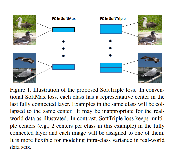
Distance metric learning (DML) is to learn the embeddings where examples from the same class are closer than examples from different classes. It can be cast as an optimization problem with triplet constraints. Due to the vast number of triplet constraints, a sampling strategy is essential for DML. With the tremendous success of deep learning in classifications, it has been applied for DML. When learning embeddings with deep neural networks (DNNs), only a mini-batch of data is available at each iteration. The set of triplet constraints has to be sampled within the mini-batch. Since a mini-batch cannot capture the neighbors in the original set well, it makes the learned embeddings sub-optimal. On the contrary, optimizing SoftMax loss, which is a classification loss, with DNN shows a superior performance in certain DML tasks. It inspires us to investigate the formulation of SoftMax. Our analysis shows that SoftMax loss is equivalent to a smoothed triplet loss where each class has a single center. In real-world data, one class can contain several local clusters rather than a single one, e.g., birds of different poses. Therefore, we propose the SoftTriple loss to extend the SoftMax loss with multiple centers for each class. Compared with conventional deep metric learning algorithms, optimizing SoftTriple loss can learn the embeddings without the sampling phase by mildly increasing the size of the last fully connected layer. Experiments on the benchmark fine-grained data sets demonstrate the effectiveness of the proposed loss function.

먼저 Conventional한 Triple Loss의 문제점은 Dataset이 Pair로 잡기 때문에 많이 진다는 것 이다. 이로 인하여 의미없는 Dataset을 많이 학습하여 Underfitting 혹은, 어려운 Dataset이 많이 발생하여 Overfitting되는 경향이 있다. 이러한 문제점을 해결하기 위하여 Sampling기법을 하여 Loss가 큰(어려운 문제)를 먼저 학습하고, Loss가 작은(쉬운)문제 순으로 해결하거나, 특정 몇몇 Sample만으로서 학습이 이루워 진다. 이러한 Triple Loss의 문제 때문에 Sampling이 수행되는데 Sampling은 Mini-Batch안에서 수행되므로, Global optimum에 도달하는 것이 아닌, Sub Optimum값으로서 학습되게 된다.

해당 논문은 이러한 문제를 해결하기 위하여, 기존에 많이 사용하던 Softmax과 TripleNet을 합치는 방법을 제시한다. 또한, Softmax는 단일 Center(Anchor)를 가지는 TripleNet과 동일하다는 것을 증명하고, 여러 Center로서 사용하였다.

여러 Center를 사용하는 이유는 1개의 Class에서도 여러개의 Cluster로서 묶을 수 있기 때문이다. 즉, Birds가 단순히 새로 분류하는 것이 아니라, 그 새안에서 여러 Characteristics를 각각 비교하여 더 Smooth하고 Performance가 좋은 Model을 만들 수 있다는 것 이다.

Introduction

Convential Distance로서 Mahalanobis Distance(\(\text{dist}_M(x_i, x_j) = (x_i - x_j)^T \text{M} (x_i - x_j)\), Appendix 참조)를 많이 사용하나, Computational Cost가 \(\text{O}(d^3)\)로서 많이 걸리게 된다.

또한 많이 사용하는 Triple Loss를 사용하게 되는 경우 Introduction에서 지적한 큰 문제점 2가지가 발생하게 된다.

1. Dataset이 N이라면, Triple Loss의 Dataset으로서는 \(\text{Anchor}(M) x \text{Same Label}(\approx (N-M)/2), \text{ Different Label}(\approx (N-M)/2)\)로서 많아지게 되어서, Computational Cost가 커지게 된다. (Balanced Dataset이라면)
2. Model Training안에서는, Mini-Batch에만 접근할 수 있으므로, Global Optimum을 찾는데에는 문제점이 발생하게 된다.(TripleNet안에서)

다음 인용구문은 Paper의 핵심이기 때문에, 원본 그대로의 내용을 전달하면 다음과 같다.

Our Analysis demonstrates that SoftMax loss is equivalent to a smoothed triplet loss. By providing a single center for each class in the last fully connected layer, the triplet constraint derived by SoftMax loss can be defined on an original example, its corresponding center and a center from a different class.
Therefore, embeddings obtained by optimizing SoftMax loss can work well as a distance metric. However, a class in real-world data can consist of multiple local clusters as illustrated in Fig. 1 and a single center is insufficient to capture the inherent structure of the data. Consequently, embeddings learned from SoftMax loss can fail in the complex scenario.
Compared with a single center, multiple ones can capture the hidden distribution of the data better due to the fact that they help to reduce the intra-class variance.
Apparently, SoftTriple loss has to determine the number of centers for each class. To alleviate this issue, we develop a strategy that sets a sufficiently large number of centers for each class at the beginning and then applies L2,1 norm to obtain a compact set of centers. We demonstrate the proposed loss on the fine-grained visual categorization tasks, where capturing local clusters is essential for good performance.

위의 구문에서 핵심을 다음과 같다.

1. Classification Model에서 많이 사용하는 Softmax는 Single Center TripleNet을 Smooth하게 표현한 것과 같다. => 생각해보면, Softmax라는 것은 하나의 Sample이 들어왔을 때, 상대적으로 어느 Class에 가깝냐를 판단하는 것 이다. 즉, 1개의 Sample이 상대적으로 Feature Sapce상에서 어느 Class와 Distance가 가까운지를 Smooth하게 Expoential Function에 표현한 것이라 할 수 있다.
2. 논문의 핵심은 1의 생각을 Base로서 Single Center가 아닌 여러 Center를 잡는 것으로서 Performance를 향상시켰다. 하나의 Class에서도 여러가지 Characteristic이 존재하게 될 것이고, 이것을 고려하게 된다면, Intra-Class간의 Hidden Space에서 Variance는 줄어들게 될 것 이다.
3. 그렇다면, 어떻게 Center수를 적절히 조절할 것인가에 대하여, 처음에는 많은 수의 Center를 지정한 뒤, \(L_{2,1}\) normalization을 통하여 실제로 필요한, Compact한 Center만 사용하는 방법을 선택하였다.

Appendix. Mahalanobis distance

$$\text{dist}_M(x_i, x_j) = (x_i - x_j)^T \text{M} (x_i - x_j)$$

• \(M\): Learned Matrix => Inverse of Covariance: \(\sum^{-1}\)

위의 식을 살펴보게 되면 Mahalanobis Distance은 Inverse of Covariance를 곱함으로 인하여 변수들 간의 Correlation등 분포를 고려하여 거리를 잴 수 있다.

만약, 모든 변수들끼리 Independent하고, Variance가 1로서 정규화 되어있다면, Euclidian Distance와 동일하다는 것을 알 수 있다.

Related Work

Conventional distance metric learning and deep metric learning

Distance metric learning 해당 논문에서는 크게 2가지로 분류하고 있다.

1. PCA와 같은 방법으로 Feature Reduction후, PSD Projections를 수행한다. 이러한 방법은 Computation Cost를 줄일 수 있는 방법이긴 하나, Embedding -> Classification이라는 2 Step을 거쳐야 되므로, Classification에 직접적으로 영향을 미치는 Embedding을 구할 수 없다. 또한, Row-Rank로서 Dimension을 줄일 수 있다는 Assumption이 필요하다.(Variance가 작은 것을 없애기 위하여)
2. 다른 방법으로는 Triplet Constraints가 있으나, 위에서 언급하였듯이, \(O(n^3)\)이라는 큰 Computation Cost가 필요하게 된다.

Deep metric learning 기본적인 Deep Learning방법으로서 Classification이 이루워 질 수 있다. 하지만, 이러한 방식은 SGD로서 Optimization이 수행되므로, Mini-Batch안에서 이루워질 수 밖에 없다. 즉, 모든 Dataset을 고려하여 Optimization을 수행할 수 없다는 것 이다. 이러한 방법을 해결하기 위해 많은 Smpling방법이 제안되었으나, 여전히 Whole Dataset을 고려할 수 없다는 문제가 발생한다. (Mini-Batch수를 늘리는 방법은 GPU Memory가 감당할 수 없다.)

Learning with proxies TripleNet을 살펴보게 되면, 기준이 되는 Anchor를 잡을 수 있다. 이러한 Anchor는 Class별 1개 혹은, 전체 1개로서 이루워지게 된다. 이러한 방식은 해당논문에서는 Softmax와 동일하다고 말하고 있다. 하지만, 여전히 Computation Cost가 높아 Sampling이 필요하게 된다. 해당 논문은 이러한 문제점을 해결하기 위하여, Sampling이 없고, Whole Dataset의 Distribution을 고려할 수 있는 SoftTriple Loss를 제안한다.

SoftTriple Loss

Analyzes the SoftMax loss and proposes the SoftTriple loss accordingly

SoftMax

• Formula: \(\text{Pr}(Y=y_i | x_i) = \frac{\text{exp}(w_{y_i}^T)x_i}{\sum_{j}^C \text{exp}(w_j^T x_i)}\) \((\text{ C:Num of Class, D: Dimension of Embedding})\)
• Loss: \(l_{\text{SoftMax}}(x_i) = -\text{log}\frac{\text{exp}(w_{y_i}^T)x_i}{\sum_{j}^C \text{exp}(w_j^T x_i)}\)
• Loss(Normalization): \(l_{\text{SoftMax}_{\text{norm}}}(x_i) = -\text{log}\frac{\text{exp}(\lambda w_{y_i}^T)x_i}{\sum_{j}^C \text{exp}(\lambda w_j^T x_i)}\) \((\lambda: \text{Scaling Factor})\)

TripleNet

• Fomula: \(\forall i, j, k \text{ } \|x_i-x_k\|_2^2 - \|x_i-x_j\|_2^2 \ge \delta\)
• Formula(i.e., \(\|x\|_2 = 1\)(Unit Length)): \(\forall i, j, k \text{ }x_i^Tx_j - x_i^Tx_k \ge \delta\)
• Loss: \(l_{triplet}(x_i, x_j, x_k) = [\gamma+x_i^Tx_k - x_k^Tx_j]_{+}\)

해당논문은 Normalization Softmax Loss가 Single Anchor를 같는 Triplenet과 같다는 것을 증명하였다.

Proposition 1.

$$l_{\text{SoftMax}_{norm}}(x_i) = \text{max}_{p \in \triangle} \lambda \sum_{j} p_j x_i^T(w_j - w_{y_i}) + H(p)$$

• \(H(p)\): Entropy Regularization

• \(p \in \mathbb{R}^c, \triangle = \{p|\sum_j p_j = 1, \forall j p_j \ge 0\}\)

위의 식을 살펴보게 되면각 새로운 p: Distribution over class를 도입하여, 해당되는 class의 probability = 1, 다른 probability는 0으로서 만들고, Entropy regularization을 더해주었다.

Proof.
K.K.T. Condition

$$p_j = \frac{\text{exp}(\lambda x_i^T(w_j-w_{y_i}))}{\sum_j \text{exp}(\lambda x_i^T (w_j - w_{y_i}))}$$

$$l_{\text{SoftMax}_{\text{norm}}}(x_i) = \lambda \sum_j p_j x_i^T (w_j - w_{y_i}) + H(p) = \text{log}(\sum_j \text{exp}(\lambda x_i^T (w_j - w_{y_i}))) = -\text{log}\frac{\text{exp}(\lambda w_{y_i}^T x_i)}{\sum_j \text{exp}(\lambda w_j^T x_i)}$$

Remark 1

$$\forall i,j, x_i^T w_{y_j} - x_i^T w_j \ge 0$$

위의 식을 살펴보게 되면, 해당 Class에 해당되는 Probability는 항상 다른 Class가 될 Probability보다 높다는 것을 알 수 있다. 위의 식을 살펴보게 되면, Triple Loss와 비슷하다는 것을 알 수 있다.

$$\forall i, j, k \text{ }x_i^Tx_j - x_i^Tx_k \ge \delta$$

즉, Softmax Loss를 Minimizing하는 방식에 Distance-Based Tasks(TripleNet)를 부여할 수 있다는 것 이다.

Remark 2
만약, Entropy Regulairzation(H(p))가 없다고 생각하면 식을 다음과 같이 적을 수 있다. (아직, Entropy Regularization에 대하여 공부하지 못하여 원문 그대로 적었습니다.)

$$\max_{p \in \triangle} \lambda \sum_j p_j x_i^T w_j - \lambda x_i^T w_{y_i}$$

$$\text{max}_j \{ x_i^T w_j\} - x_i w_{y_i}$$

Explicitly, it punishes the triplet with the most violation and becomes zero when the nearest neighbor of xi is the corresponding center wyi. The entropy regularizer reduces the influence from outliers and makes the loss more robust. λ trades between the hardness of triplets and the regularizer. Moreover, minimizing the maximal entropy can make the distribution concentrated and further push the example away from irrelevant centers, which implies a large margin property.

Appendix. Entropy Regularization
Understanding the Impact of Entropy on Policy Optimization
https://arxiv.org/pdf/1811.11214.pdf

Multiple Centers

이제 각각의 Class가 K개의 Centers를 가지고 있으면, Input \(x_i\)와 각각의 Class안의 K개의 Center와의 Similarity는 다음과 같이 표현 가능하다.

$$S_{i,c} = \text{max}_k x_i^T w_c^k$$

다른 표현으로는 다음과 같이 생각할 수 있다.

$$\text{min}_{z \in \mathbb{R}^K}\| [w_c^1, ..., w_c^K]z-x_i \|_2$$

즉, Class간의 Similarity를 최대화 하면서, Class안에서의 K개의 Center로서 Cluster효과를 보겠다는 것 이다. 따라서 논문에서 제시하는 Intra Class간의 Variance를 줄일 수 있는 효과를 확인할 수 있다.

위의 식을 Triple Loss로서 표현하면 다음과 같다.

$$\forall j, S_{i,y_i} - S_{i,j} \ge 0$$

위의 식에서 Small Margin이 존재한다고 정의하면 식은 다음과 같이 바꿀 수 있다.

$$\forall j, S_{i,y_i} - S_{i,j} \ge \delta$$

위의 식을 다시 Proposition 1으로서 나타내면 다음과 같다.

$$l_{\text{HardTriple}}(x_i) = \text{max}_{p \in \triangle}\lambda(\sum_{j \neq y_i}p_j (S_{i,j} - (S_{i,y_i}-\delta))+p_{y_i}(S_{i,y_i}-\delta-(S_{i,y_i}-\delta)))+H(p)$$

$$= -\text{log} \frac{\text{exp}(\lambda(S_{i,y_i}-\delta))}{\text{exp}(\lambda(S_{i,y_i}-\delta))+\sum_{j\neq y_i}\text{exp}(\lambda S_{i,j})}$$

위의 식에서 Similarity를 구하는 식을 살펴보게 되면, \(S_{i,c} = \text{max}_k x_i^T w_c^k\)로서 Max Operator이다. 이러한 식은, Not Smooth하므로 Sensitive하다. 따라서 해당 논문을 이러한 식에 Entropy Regularization을 도입하여 Smooth한 형태로 바꾸었다.

$$\text{max}_{q \in \triangle} \sum_{k} q_k x_i^T w_k^k \rightarrow \text{max}_{q \in \triangle} \sum_{k} q_k x_i^T w_k^k + \gamma H(q)$$

K.K.T. Condition => Closed form

$$q_k = \frac{\text{exp}(\frac{1}{\gamma}x_i^T w_c^k)}{\sum_{k}\text{exp}(\frac{1}{\gamma}x_i^T w_c^k)}$$

위와 같은 식을 병형하면, Similarity는 다음과 같이 변형된다.

$$S_{i,c} = x_i^T w_c^k \rightarrow S^{'}_{i,c} = \sum_{k} \frac{\text{exp}(\frac{1}{\gamma}x_i^T w_c^k)}{\sum_{k} \text{exp}(\frac{1}{\gamma}x_i^T w_c^k)} x_i^T w_c^k$$

최종적인 Loss Function은 다음과 같이 이루워 진다.

$$l_{\text{SoftTriple}}(x_i) = -\text{log} \frac{\text{exp}(\lambda(S^{'}_{i,y_i}-\delta))}{\text{exp}(\lambda(S^{'}_{i,y_i}-\delta))+\sum_{j\neq y_i}\text{exp}(\lambda S^{'}_{i,j})}$$

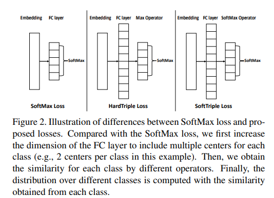
Compare to Softmax Loss & HardTriple Loss & SoftTriple Loss

Adaptive Number of Centers

논문에서 계속해서 강조하는 것은 Softmax Loss는 K(Number of Centers) = 1이다. 이러한 Softmax Loss는 Efficient하지만 Ineffective이다. Hard Triple Loss는 K = N으로서, Inefficient하지만 Effective하다.

SoftTriple Loss는 이러한 K를 어떻게 선언할 것인지가 중요하다.
해당 논문은 이러한 문제를 해결하기 위하여 \(L_{2,1}\) norm을 적용하였다.

만약, \(w_j^t\)라는 j Class의 Center가 있다고 가정하면, 우리는 다음과 같은 Matrix를 정의할 수 있다.

$$M_j^t = [w_j^1-w_j^t, ..., w_j^K - w_j^t]^T$$

위의 상황에서 \(w_j^s\)라는 Center와 현재, \(w_j^t\)의 Center가 유사하다면, \(\| w_j^s - w_j^t\|_2 = 0\)이 될 것이다.

이러한 방식은 L2 norm과 같은 형식이고 다음과 같이 식을 정리할 수 있다.

$$\|M_j^t\|_{2,1} = \sum_{s}^K \|w_j^s - w_j^t \|_2$$

위의 식을 Multiple Center에 모두 적용하면, 다음과 같이 적을 수 있다.

$$\text{R} (w_j^1, ... , w_j^K) = \sum_{t}^K \| M_j^t\|_{2,1} $$

$$ = \sum_{t=1}^K \sum_{s=t+1}^K \sqrt{2-2{w_j^s}^T w_j^t}$$

즉, 각 Class의 Center를 기준으로 비슷한 Class로서 Cluster하는 Center는 합치겠다는 의미와 같다.

위의 Regularization을 모든 Class에 적용하면, 최종적인 LossFunction은 다음과 같다.

$$\text{min} \frac{1}{N} \sum_{i} l_{\text{SoftTriple}}(x_i) + \frac{\tau \sum_{j}^C \text{R}(w_j^1,...,w_j^K)}{CK(K-1)}$$

• \(N: \text{Num of Dataset}, C: \text{Num of Class}, K: \text{Num of Center}\)

• \(l_{\text{SoftTriple}}(x_i) = -\text{log} \frac{\text{exp}(\lambda(S^{'}_{i,y_i}-\delta))}{\text{exp}(\lambda(S^{'}_{i,y_i}-\delta))+\sum_{j\neq y_i}\text{exp}(\lambda S^{'}_{i,j})}\)

• \(S^{'}_{i,c} = \sum_{k} \frac{\text{exp}(\frac{1}{\gamma}x_i^T w_c^k)}{\sum_{k} \text{exp}(\frac{1}{\gamma}x_i^T w_c^k)} x_i^T w_c^k\)

• \(\text{R} (w_j^1, ... , w_j^K) = \sum_{t=1}^K \sum_{s=t+1}^K \sqrt{2-2{w_j^s}^T w_j^t}\)

Code

https://github.com/idstcv/SoftTriple/blob/master/loss/SoftTriple.py

Hyper Paramter

• Lambda: \(\lambda\): For Scaling Factor
• Gamma: \(\gamma\): For Similarity => SoftTriple
• Tau: \(\tau\): For Regularization rate
• Delta: \(\delta\): For Margin
• K: Number of Center(Each Class)

Parameter

• dim: For FC Layer(Previous Hidden Layer Output Shape) => \(w_c^k\)
• weight: Mask For Regularization => \(\sum_{t=1}^K \sum_{s=t+1}^K\)
• cN: Number of Class

Description of Code

• input = F.normalize(input, p=2, dim=1): Normalization Input => Change to Unit Vector (\(x_i\))
• centers = F.normalize(self.fc, p=2, dim=0): Normalization Weight => Change to Unit Vector (\(w_j^c\))
• simInd = input.matmul(centers), simStruc = simInd.reshape(-1, self.cN, self.K): Soft Similarity \(x_i^T w_c^k\)
• prob = F.softmax(simStruc*self.gamma, dim=2): Soft Similarity \(\frac{\text{exp}(\frac{1}{\gamma}x_i^T w_c^k)}{\sum_{k} \text{exp}(\frac{1}{\gamma}x_i^T w_c^k)}\)
• simClass = torch.sum(prob*simStruc, dim=2): Soft Similarity \(S^{'}_{i,c} = \sum_{k} \frac{\text{exp}(\frac{1}{\gamma}x_i^T w_c^k)}{\sum_{k} \text{exp}(\frac{1}{\gamma}x_i^T w_c^k)} x_i^T w_c^k\)
• marginM = torch.zeros(simClass.shape).cuda(): Margin \(\delta\)
• lossClassify = F.cross_entropy(self.la*(simClass-marginM), target): Loss of SoftTriple \(l_{\text{SoftTriple}}(x_i) = -\text{log} \frac{\text{exp}(\lambda(S^{'}_{i,y_i}-\delta))}{\text{exp}(\lambda(S^{'}_{i,y_i}-\delta))+\sum_{j\neq y_i}\text{exp}(\lambda S^{'}_{i,j})}\)
• simCenter = centers.t().matmul(centers): Regularization Term \(w_j^t w_j\)
• reg = torch.sum(torch.sqrt(2.0+1e-5-2.* simCenter[self.weight]))/(self.cN * self.K * (self.K-1.)): Regularization Term \(\frac{\sum_{j}^C \text{R}(w_j^1,...,w_j^K)}{CK(K-1)}\)
  • simCenter[self.weight]: \({w_j^s}^T w_j^t\)

class SoftTriple(nn.Module):
    def __init__(self, la, gamma, tau, margin, dim, cN, K):
        super(SoftTriple, self).__init__()
        self.la = la
        self.gamma = 1./gamma
        self.tau = tau
        self.margin = margin
        self.cN = cN
        self.K = K
        self.fc = Parameter(torch.Tensor(dim, cN*K))
        self.weight = torch.zeros(cN*K, cN*K, dtype=torch.bool).cuda()
        for i in range(0, cN):
            for j in range(0, K):
                self.weight[i*K+j, i*K+j+1:(i+1)*K] = 1
        init.kaiming_uniform_(self.fc, a=math.sqrt(5))
        return

    def forward(self, input, target):
        centers = F.normalize(self.fc, p=2, dim=0)
        simInd = input.matmul(centers)
        simStruc = simInd.reshape(-1, self.cN, self.K)
        prob = F.softmax(simStruc*self.gamma, dim=2)
        simClass = torch.sum(prob*simStruc, dim=2)
        marginM = torch.zeros(simClass.shape).cuda()
        marginM[torch.arange(0, marginM.shape[0]), target] = self.margin
        lossClassify = F.cross_entropy(self.la*(simClass-marginM), target)
        if self.tau > 0 and self.K > 1:
            simCenter = centers.t().matmul(centers)
            reg = torch.sum(torch.sqrt(2.0+1e-5-2.*simCenter[self.weight]))/(self.cN*self.K*(self.K-1.))
            return lossClassify+self.tau*reg
        else:
            return lossClassify

Experiments & Conclusion

Experiment

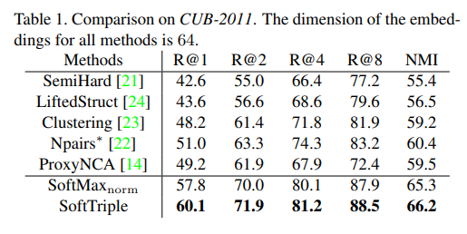
Comparison on CUB-2011에서 기존의 방식들보다 휼륭한 Performance를 보여준다. 특히, Softmax norm보다 성능이 좋은 것을 보여주고 있다.

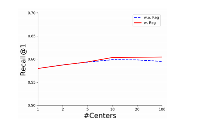위의 결과는 Reguralization(\(\frac{\tau \sum_{j}^C \text{R}(w_j^1,...,w_j^K)}{CK(K-1)}\))에 대하여 비교한 것 이다. Regularization이 없는 경우에는 일정 K개의 개수개가 넘어가면 Performance가 좋지 않지만, Regularization을 거는 경우, Compact한 Center만 남기 때문에, Performance의 하락이 덜한 것을 알 수 있다.

Conclusion

Sampling triplets from a mini-batch of data can degrade the performance of deep metric learning due to its poor coverage over the whole data set. To address the problem, we propose the novel SoftTriple loss to learn the embeddings without sampling. By representing each class with multiple centers, the loss can be optimized with triplets defined with the similarities between the original examples and classes. Since centers are encoded in the last fully connected layer, we can learn embeddings with the standard SGD training pipeline for classification and eliminate the sampling phase. The consistent improvement from SoftTriple over fine-grained benchmark data sets confirms the effectiveness of the proposed loss function. Since SoftMax loss is prevalently applied for classification, SoftTriple loss can also be applicable for that. Evaluating SoftTriple on the classification task can be our future work.

아직, Classification까지, End-to-End로서 구현하지는 못하고, Future Work로 남겨두었다. 실제 Code에서도 Embedding후, KNN으로서 평가하는 것을 알 수 있다.