Paper10. PCGrad

8 minute read

Gradient Surgery for Multi-Task Learning

Gradient Surgery for Multi-Task Learning (https://proceedings.neurips.cc/paper/2020/file/3fe78a8acf5fda99de95303940a2420c-Paper.pdf)

Abstract

While deep learning and deep reinforcement learning (RL) systems have demonstrated impressive results in domains such as image classification, game playing, and robotic control, data efficiency remains a major challenge. Multi-task learning has emerged as a promising approach for sharing structure across multiple tasks to enable more efficient learning. However, the multi-task setting presents a number of optimization challenges, making it difficult to realize large efficiency gains compared to learning tasks independently. The reasons why multi-task learning is so challenging compared to single-task learning are not fully understood. In this work, we identify a set of three conditions of the multi-task optimization landscape that cause detrimental gradient interference, and develop a simple yet general approach for avoiding such interference between task gradients. We propose a form of gradient surgery that projects a task’s gradient onto the normal plane of the gradient of any other task that has a conflicting gradient. On a series of challenging multi-task supervised and multi-task RL problems, this approach leads to substantial gains in efficiency and performance. Further, it is model-agnostic and can be combined with previously-proposed multi-task architectures for enhanced performance.

Multi-Task Domain에서 Model을 Training하는 것은 어렵다.
이를 해결하기 위한 방법으로서, Conflicing Gradients에서 하나의 Gradient를 Projection하는 방향으로서 Optimization을 실시하여 해결하는 방법을 제안
이러한 방법은 Multi Task Architecture어디에서도 사용할 수 있도록 제공가능

Introduction

Learning multiple tasks all at once results is a difficult optimization problem, sometimes leading to worse overall performance and data efficiency compared to learning tasks individually. If we could tackle the optimization challenges of multi-task learning effectively, we may be able to actually realize the hypothesized benefits of multi-task learning without the cost in final performance. Prior work has described varying learning speeds of different tasks and plateaus in the optimization landscape as potential causes, whereas a range of other works have focused on the model architecture. In this work, we instead hypothesize that one of the main optimization issues in multi-task learning arises from gradients from different tasks conflicting with one another in a way that is detrimental to making progress.
If two gradients are conflicting, we alter the gradients by projecting each onto the normal plane of the other, preventing the interfering components of the gradient from being applied to the network. We refer to this particular form of gradient surgery as projecting conflicting gradients (PCGrad)

Probelm of MuultiTask

png

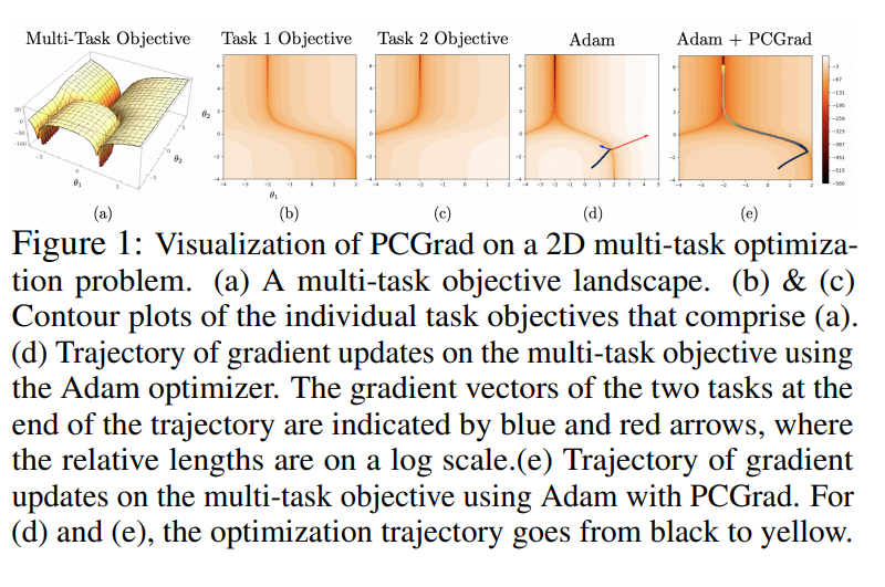
위의 사진을 살펴보게 되면, 논문에서 주장하는 Multi-Task Learning이 어려운 이유를 알 수 있다. 각각의 Task가 다른 방향으로 Optimization되어야 하는 경우, Gradient가 충돌을 일으키면서 학습이 잘 되지 않는 다는 것 이다.
이것을 해결하기 위한 이전 연구들은 각각의 Task의 Learning Rate를 조절함으로서 해결하였다.

Previous Method

DANN_TF Model을 살펴보면 이전 방식의 Multi-Task Learning을 알 수 있다.
png

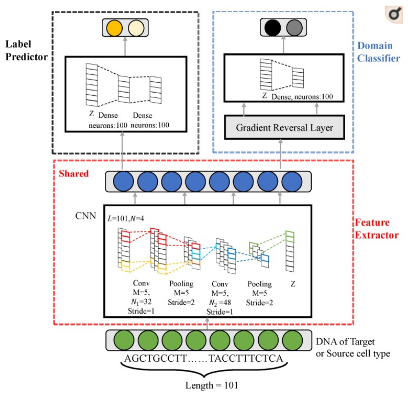
DANN TF의 Task는 크게 2개이다. Task 1: Classification, Task 2: Remove Batch Effect => 이 2가지 Task를 Upate하기 위하여 Domain Classifier Learning Rate를 작게 주거나, Sigmoid형식으로 차차 올리는 방식을 택하여 Learning을 하였다.

PCGrad

해당 논문에서는 Learning Rate를 변경시키는 방법이 아닌 두개의 Gradient가 Conflicting하는 상황에서 각각의 Gradient를 Projection하여 절충하는 방향으로 Update시키는 gradient surgery as projecting conflicting gradients (PCGrad)을 제안한다.

Preliminaries: Problem and Notation

$\theta$: Parameters of a model $f_{\theta}$
$p(\tau)$: Distrubution of Tasks
$\min_{\theta} E_{T_i ~ p(\tau)}[L_i(\theta)]$: Optimization // $L_i(\theta)$: Loss function for i-th task($\tau_i$)
$L(\theta) = \sum_{i}L_i(\theta)$: Multi-Task Loss
$g_i = \nabla L_i(\theta)$: Gradient of each Task

The Tragic Triad: Conflicting Gradients, Dominating Gradients, High Curvature

논문에서는 먼저 Multi-Task Learning이 잘 작동하지 않는 Condition 3가지에 대하여 정의하였다.

When gradients from multiple tasks are in conflict with one another => Gradient가 충돌하는 경우
When the difference in gradient magnitudes is large, leading to some task gradients dominating others => Gradient의 Scale이 달라서 다른 Gradient가 무시되는 경우
When there is high curvature in the multi-task optimization landscape => High Curvature로 인하여 수렴을 못하는 경우

위의 각각의 3가지 상황을 정량화 하기 위하여 Definition을 정의하였다.

Definition 1: Define $\phi_{i,j}$ as angle between two task gradients $g_i$ and $g_j$. Define the gradient as conflicting when $\text{cos} \phi_{i,j} <0$

Definition 2: Define the gradient magnitude smilarity between two gradients $g_i$ and $g_j$ as $\Phi(g_i, g_j) = \frac{2 ||g_i||_2 ||g_j||_2}{||g_i||_2^2 ||g_j||_2^2}$

Definition 3: Define the multi-task curvature as $H(L;\theta,\theta^{'}) = \int_{0}^{1} \nabla L(\theta)^T \nabla^2 L(\theta + \alpha(\theta^{'}-\theta))\nabla L(\theta) da$, which is the averaged curvature of L between $\theta$ and $\theta^{'}$ at the current and next iteration, characterize the optimization landscape as having high cuvature.

When $H(L;\theta,\theta^{'})>C$ for some large positive constant C, for model paramters $\theta$ and $\theta^{'}$ at the current and next iteration, we characterize the optimization landscape as having high curvature.

PCGrad: Project Conflicting Gradients

png

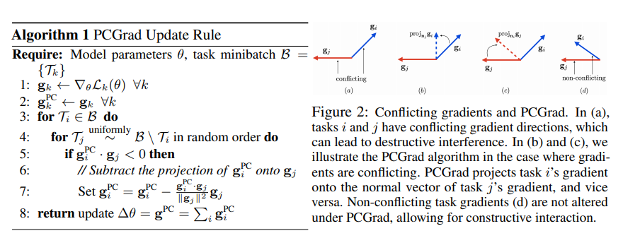
PCGrad Update Rule

Determines whether $g_i$ conflicts with $g_j$ by computing the cosine similarity between vectors $g_i$ and $g_j$, where negative values indicate conflicting gradients
if the cosine similarity is negative, replace $g_i$ by its projection onto the normal plane of $g_j:g_i = g_i - \frac{g_i \cdot g_j}{||g_j||^2}g_j$. If the gradients are not in conflict, i.e. cosine similarity is non-negative, the original gradient $g_i$ remains unaltered.
PCGrad repeats this process across all of the other tasks sampled in random over form the current batch $\tau_i \forall j \neq i$, resulting in the gradient $g_i^{PC}$ that is applied for task $\tau_i$

PCGrad는 간단하다. 각각의 Gradient간의 Conflict의 Condition은 Cosine Similarity가 Negative인 경우이고, 이러한 경우에 각각의 Gradient에서 Conflict하는 부분을 제거한다. Conflict한 부분은 각각의 Gradient의 Projection하여 알아낸다.

Theoretical Analysis of PCGrad

먼저 Paper에서 각각의 Condition에서 Loss에 대해 분석하기 위하여 다음과 같이 2개의 Task에 대하여 정의하였다.

Definition 4.: Consider two task loss functions $L_1: \mathbb{R}^n \rightarrow \mathbb{R}$ and $L_2: \mathbb{R}^n \rightarrow \mathbb{R}$. Paper define the two-task learning objective as $L(\theta) = L_1(\theta)+L_2(\theta)$ for all $\theta \in \mathbb{R}^n$, where $g_1 = \nabla L_1(\theta), g_2 = \nabla L_2(\theta)$, and $g=g_1+g_2$

Converge of PCGrad in convex setting, under standard assumptions in Theorm 1.
Theorm 1.의 가정 + Convex인 경우에 Converge하는 것을 증명하였다.

Theorem 1.: Assume $L_1$ and $L_2$ are convex and differentiable. Suppose the gradient of $L$ is Lipschitz with $L > 0$. Then, the PCGrad update rule with step size $t \leq \frac{1}{L}$ will converge to either a location in the optimization landscape where $\text{cos}(\phi_{12}) = -1$ or the optimal value $L(\theta^{*})$

먼저 증명을 하기 전에 알아야 하는 Function은 Lipschitz Funciton이다.

Lipschitz Function
Let a function $f: [a,b] \rightarrow \mathbb{R}$ s.t. for some constant $\mathbb{M}$ and for all $x,y \in [a,b], |f(x)-f(y)| \leq M|x-y|$

위의 식을 살펴보게 되면 Lipschitz Function이라는 것은 두 점 사이의 거리를 일정 이상으로 증가시키지 않는 함수이다.

Lipschitz constant
For funtions $f:[a,b] \rightarrow \mathbb{R}$, it denotes the smallest constant $\mathbb{M} > 0$ in Lipschitz condition, namely the nonnegative number

$$\text{sup}_{x\neq y}\frac{|f(y)-f(x)|}{|y-x|} \leq M$$

If the domain of f is an interval, the function is everywhere differentiable and the derivation is bounded, then is is esasy to see that the Lipschitz constant of f euqals

$$\text{sup}_x |f^{'}(x)| \leq K, K \geq 0$$

참조: Wikipedia

즉, Lipschitz Function은 두 점 사이의 거리를 일정 이상으로 증가시키지 않는 함수이며, 미분값이 0보다 크며 일정 값보다 항상 일정 값보다 작다

Proof
Assumption: $\nabla L$ is Lipschitz continuous with constant $L$ implies that $\nabla^2 L(\theta) - LI$is a negative semi-definite matrix. Using this fact, we can perform a quardratic expansion of $L$ around $L(\theta)$ and obtain the following ineuqality.

즉, Therom1 => Gradient Vanishing or Gradient Exploding이 없이 진행된다. Convex => Gradient Descent가 잘 이루워 진다.

$$L(\theta^{+}) \leq L(\theta) + \nabla L(\theta)^T(\theta^{+}-\theta) + \frac{1}{2}\nabla^2 L(\theta)||\theta^{+}-\theta||^2$$

$$\leq L(\theta) + \nabla L(\theta)^T(\theta^{+}-\theta) + \frac{1}{2}L||\theta^{+}-\theta||^2$$

PCGGrad update by letting $\theta^{+} = \theta -t\cdot (g-\frac{g_1 \cdot g_2}{||g_1||^2}g_1-\frac{g_1 \cdot g_2}{||g_2||^2}g_2)$

$$L(\theta^{+}) \leq L(\theta) + t\cdot g^T(-g+\frac{g_1 \cdot g_2}{||g_1||^2}g_1+\frac{g_1 \cdot g_2}{||g_1||^2}g_2)+\frac{1}{2}Lt^2||g-\frac{g_1 \cdot g_2}{||g_1||^2}g_1-\frac{g_1 \cdot g_2}{||g_2||^2}g_2||^2$$

$$(\text{Expanding, using the identity} g=g_1+g_2)$$

$$=L(\theta)+t(-||g_1||^2-||g_2||^2+\frac{(g_1\cdot g_2)^2}{||g_1||^2}+\frac{(g_1\cdot g_2)^2}{||g_2||^2})+\frac{1}{2}Lt^2||g_1+g_2-\frac{g_1 \cdot g_2}{||g_1||^2}g_1-\frac{g_1 \cdot g_2}{||g_2||^2}g_2||^2$$

$$\text{Expanding further and re-arranging terms}$$

$$L(\theta) - (t-\frac{1}{2}Lt^2)(||g_1||^2+||g_2||^2-\frac{(g_1 \cdot g_2)^2}{||g_1||^2}-\frac{(g_1 \cdot g_2)^2}{||g_2||^2})-Lt^2(g_1 \cdot g_2 - \frac{(g_1 \cdot g_2)^2}{||g_2||^2 ||g_2||^2}g_1 \cdot g_2)$$

$$\text{Using the identity }cos(\phi_{12}) = \frac{g_1 \cdot g_2}{||g_1||||g_2||}$$

$$=L(\theta) - (t-\frac{1}{2}Lt^2)[(1-\text{cos}^2(\phi_{12})||g_1||^2+(1-\text{cos}^2(\phi_{12})||g_2||^2)]-Lt^2(1-\text{cos}^2(\phi_{12}))||g_1||||g_2||\text{cos}(\phi_{12})$$

$$\text{Condition 1.} -(1-\frac{1}{2}Lt) = \frac{1}{2}Lt-1 \leq \frac{1}{2}L(1/L)-1 = -\frac{1}{2}$$

$$\text{Condition 2.} Lt^2 \leq t (\because t \leq \frac{1}{L})$$

Using Last expression above

$$L(\theta^{+}) \leq L(\theta) -\frac{1}{2} t[(1-\text{cos}^2(\phi_{12}))||g_1||^2+(1-\text{cos}^2(\phi_{12}))||g_2||^2]-t(1-\text{cos}^2(\phi_{12}))||g_1||||g_2||\text{cos}(\phi_{12})$$

$$=L(\theta)-\frac{1}{2}t(1-\text{cos}^2(\phi_{12}))[||g_1||^2+2||g_1||||g_2||\text{cos}(\phi_{12})+||g_2||^2]$$

$$=L(\theta)-\frac{1}{2}t(1-\text{cos}^2(\phi_{12}))[||g_1||^2+2g_1 \cdot g_2 + ||g_2||^2]$$

$$=L(\theta) - \frac{1}{2} t(1-\text{cos}^2 (\phi_{12}))||g_1+g_2||^2$$

$$=L(\theta)-\frac{1}{2}t(1-\text{cos}^2(\phi_{12}))||g||^2$$

즉, $\frac{1}{2}t(1-\text{cos}^2(\phi_{12}))||g||^2 \geq 0$을 만족한다. 0인 경우는 2가지의 경우를 생각할 수 있다.

Condition 1. $||g||=0$
||g||=0인 경우로서, $g = g_1+g_2 = \nabla L_1 + \nabla L_2 = 0$으로 Loss의 Gradient가 0인 경우(=Local Minumum or Global Minimum) 이다.

Condition 2. $\text{cos}(\phi_{12})=-1$
위의 경우에는 2 Gradient가 서로 완전히 Conflict한 경우이다. 이러한 경우는 하나의 Sample에서는 이루워질 수 있으나, SGD혹은 Batch를 사용하게 되는 실제 Pratice의 경우에는 거의 발생하지 않는다.

Probelm. $\text{cos}^2(\phi_{12}) \approx -1$
$\text{cos}^2(\phi_{12})$의 값이 -1에 가까울 수록 Converge속도는 느려지는 경향을 보일 수 있으나, 실제 Experiment는 그러한 결과를 보이지 않았다. => Experiment: NYU Dataset v2

또한, Non-Convex이고, Multi-Task Learning이 잘 작동하지 않는 Condition3가지에 대하여 모두 잘 작동하는 것은 Paper에서는 수식으로 증명하였다. Appendix 참조

PCGrad in Practice

PCGrad를 실제 Batch단위로서 이루워지며, Model-Agnostic이고, 어떠한 Architecture에서 사용될 수 있다고 한다. Code는 실제로 Pytorch-PCGrad에서 제공한다.

실제 Code에서 중요한 부분은 다음과 같다.

def _project_conflicting(self, grads, shapes=None):
    pc_grad, num_task = copy.deepcopy(grads), len(grads)
    for g_i in pc_grad:
        random.shuffle(grads)
        for g_j in grads:
            g_i_g_j = torch.dot(g_i, g_j)
            if g_i_g_j < 0:
                g_i -= (g_i_g_j) * g_j / (g_j.norm()**2)
    pc_grad = torch.stack(pc_grad).mean(dim=0)
    return pc_grad

위의 Code를 보게 되면, 각각의 들어오는 Gradients에 대하여 Cosine Similarity를 torch.dot로서 계산된다. 또한 위의 Cosine Similarity의 Gradients가 반대가 되는 경우 즉, Gradients끼리 Conflict한 경우에 Projection하여 Conflict되는 부분을 제거한다.

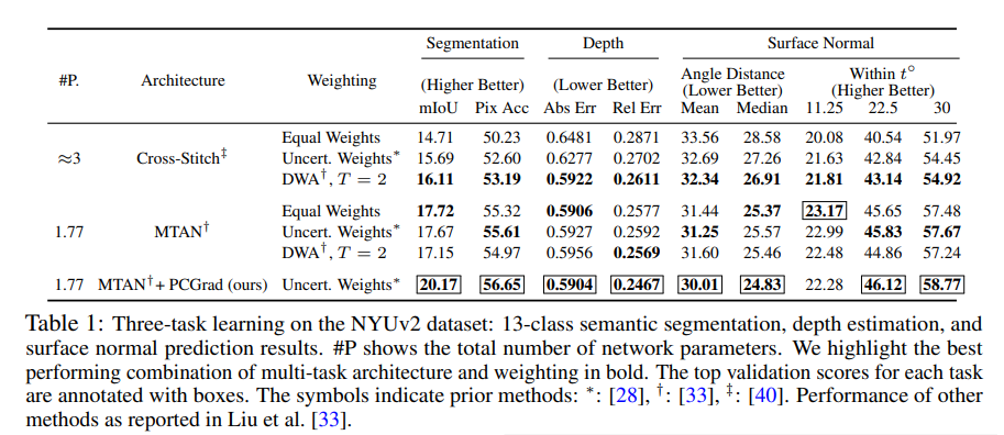
Experiment

NYU Dataset v2: https://cs.nyu.edu/~silberman/datasets/nyu_depth_v2.html
png

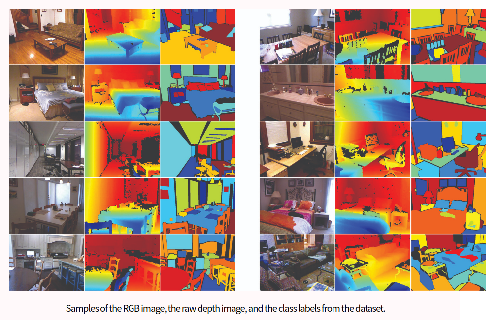
데이터셋을 살펴보게 되면, Depth와 Segmenation등의 Multi-Task를 할 수 있는 Dataset이다.
Paper의 결과를 살펴보면, 기존의 Performance가 좋은 Architecture에 PCGrad를 적용함으로서 Performance가 좋아지는 것을 살펴볼 수 있다. png

Appendix에서 살펴본, 각각의 Training과정을 살펴보면 다음과 같다. png

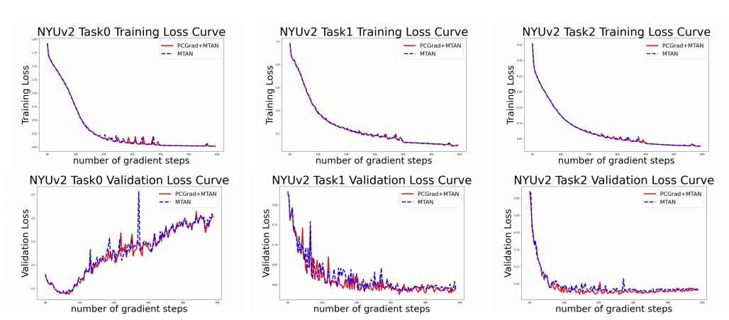
해당 논문에서 다음과 같은 결과를 Appendix로 첨부하는 이유는 Conflict한 부분을 없앰으로 인하여 Converage가 늦어질 수 있다는 단점이 존재하기 때문이다. 하지만, 실제로 적용하면 다음과 같이 기존 Method와 비슷 혹은 빠르게 Converge하고, Loss부분에서는 더 적은 것을 확인할 수 있다.

Appendix: Curvature

Curvature refers to how fast the function curves upwards when you move in a given direction. In directions of high curvature, you want to take a small step, because you can overshoot very quickly.

위의 인용은 cs.toronto.edu에서 참조하였다.
즉, High Curvature을 해결하기 위한 방법은 크게 2가지이다.

Normalization을 실시한다.
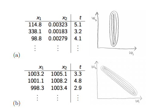위의 그림을 살펴보면 알 수 있다. 우리는 모든 Feature의 중요도를 동일 시 하기 위하여 normalization을 취한다. 라고 많이 배운다. 이것이 의미하는 것은 결국에는 Curvature를 맞춰주어서 동일한 Direction을 지정하고 Update시에 동일한 만큼 변한다고 이야기할 수 있다.
Learning Rate를 작게 준다. => Normalziation을 실시함에도 불고하고 High Curvature이면 어쩔 수 없이 Learning Rate를 작게 주어서 Minimum을 찾아내는 작업을 실시하여야 한다.

또한, 이런 의미 말고, blog.paperspace.com를 살펴보면 pathological curvature에 대해서 이야기 한다.
이 Post는 Optimization시 Pathological Curvature를 고려하면 더 빠르게 Global Optimum에 도달할 수 있다고 이야기 하고 있고, 이에 대한 방법으로서, Adam, RMS Prop, AdaGrad등을 이야기 하고 있다.

Share on

Twitter Facebook LinkedIn

JeongYong Hwang