Paper16-1. Unsupervised Feature Learning via Non-Parametric Instance Discrimination

Unsupervised Feature Learning via Non-Parametric Instance Discrimination

출처: Unsupervised Feature Learning via Non-Parametric Instance Discrimination
코드: zhirongw Github

Abstract

Neural net classifiers trained on data with annotated class labels can also capture apparent visual similarity among categories without being directed to do so. We study whether this observation can be extended beyond the conventional domain of supervised learning: Can we learn a good feature representation that captures apparent similarity among instances, instead of classes, by merely asking the feature to be discriminative of individual instances?
We formulate this intuition as a non-parametric classification problem at the instance-level, and use noisecontrastive estimation to tackle the computational challenges imposed by the large number of instance classes.
Our experimental results demonstrate that, under unsupervised learning settings, our method surpasses the stateof-the-art on ImageNet classification by a large margin. Our method is also remarkable for consistently improving test performance with more training data and better network architectures. By fine-tuning the learned feature, we further obtain competitive results for semi-supervised learning and object detection tasks. Our non-parametric model is highly compact: With 128 features per image, our method requires only 600MB storage for a million images, enabling fast nearest neighbour retrieval at the run time

해당논문에서 던지는 가장 Main이 되는 Idea는 Supervised Classification의 결과를 보게 되면, Input Image와 비슷한 다른 Class를 Input Image와 다른 Class보다 Probability를 높게 출력하도록 학습된다는 것 이다. 이러한 생각을 extend하면, 각각의 Input을 Class로서 생각하고 학습을 하게 되면, Latent Representation에서 비슷한 Image끼리는 가까운 Distance에 위치하고 되고, 다른 Image에는 먼 Distance에 위치하게 되는 Contrastive Loss와 같은 결과를 얻을 수 있다는 것 이다. 결과적으로 Label정보가 들어가지 않는 Non-parametric Classification으로서 Parametric Classification의 효과를 얻을 수 있고, Experiment결과 Performance가 더 좋다는 결과를 보여준다. 또한, 이러한 Constrastive Loss의 문제점인 Dataset을 Pair고 잡아야 된다는 것에 대해서 Memory Bank를 사용하여 효과적으로 해결하였다.

Introduction

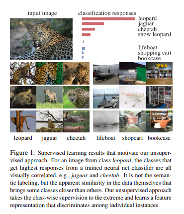
먼저 위의 그림은 Supervised Classification의 결과이다. Input Image을 Leopard로서 예측하고 있고, 2번째로는 jaguar, 가장 닮지 않은 것은 bookcase라고 예측하고 있다. 또한 대부분의 Supervised Classification의 결과중 Top-5 Classification의 결과는 Top-1 Classification의 결과보다 Error가 매우 낮은 것을 살펴볼 수 있다. 즉, Visual상 비슷한 Input끼리는 같은 Class라고 판단할 확률은 높아지게 된다는 것 이다.

이러한 결과로서 해당 논문에서는, “Label정보로서 Model을 학습하는 것은 다른 어떠한 Loss(e.g.비슷한 Image끼리는 가까워지게 학습)를 추가하지 않아도 비슷한 Image끼리 비슷한 Latent Representation으로서 나타내게 된다. \(\rightarrow\) 각각의 Input을 하나의 Class로서 생각하고 학습하게 되는 경우, 자연스럽게 비슷한 Input끼리 Latent Representation에서 위치하게 될 것이다”라는 가정을 하게되고, Experiment를 진행하였다.

해당 가정에서 문제점은 각각의 Input을 모두 Class로서 생각한다는 것 이다. 즉, 1.2 million의 Dataset을 사용하는 경우, Class는 그 개수와 같아지게 되고 Computation Cost가 너무 높아진다는 단점이 생기게 된다. 해당 논문에서는 이러한 문제점을 해결하기 위하여 noise-contrastive estimation(NCE)을 사용하였다.

Approach

Notation

• \(x\): Input
• \(n\): Number of Sample
• \(f_{\theta}(\cdot)\): DNN(=Encoder)
• \(v = f_{\theta}(x)\): Latent Representation
• \(d_{\theta}(x,y) = \|f_{\theta}(x) - f_{\theta}(y)\|\): Similarity

Non-Parametric Softmax Classifier

Parametric Classifier
기존에 Parametric Classifier을 살펴보면 다음과 같다.

$$P(i|v) = \frac{\text{exp}(w_i^T v)}{\sum_{j=1}^n \text{exp}(w_j^T v)}$$

\(w\)가 Latent Representation \(\rightarrow\) Label로 Mapping하는 Weight라고 하였을 때, Softmax를 취한 Probability이다.

Non-Parametric Classifier
해당 논문에서 제안하는 Non-Parametric Classifier을 살펴보면 다음과 같다.

$$P(i|v) = \frac{\text{exp}(v_i^T v/\tau)}{\sum_{j=1}^n \text{exp}(v_j^T v/\tau)} \text{ .s.t. }\|v\|=1 (\text{L2 Normalization layer})$$

$$\tau: \text{Temperature parameter}$$

\(w \rightarrow v\)로서 바꾸어서 Latent Representation에서 Similarity를 Probability로서 나타낸 것 이다.

해당 Classifier를 학습하기 위한 Loss Function은 다음과 같다.

$$J(\theta) = -\sum_{i=1}^n \text{log}(P(i|f_{\theta}(x_i)))$$

Learning with A Memory Bank
\(p(i|v)\)를 계산하기 위해서는 모든 \(v_i(i=1, \cdots, n)\)가 필요하게 된다. 따라서 매번 \(f_{\theta}(x_i)\)를 계산해야 하므로 Computation Cost가 많이 소모된다.

이러한 문제를 해결하기 위하여 해당논문에서는 Momory Bank \(V=\{v_j\}\)을 제안한다. \(f_{\theta}(x_i) = f_i \rightarrow v_i\)로서 Mapping된다.
해당 과정은 아래 Figure와 같다. 출처: 2-chae 블로그

해당논문에서는 Parameter인 \(\theta\)뿐만 아니라, \(f_i\)도 같이 최적화 된다 라고 얘기하고 있다.

참조: \(f_i\)는 Parameter로서 학습할 수 없는데 왜 최적화 된다고 하는 것 인가?
EX) Number of Dataset이 12만개라고 가정하자. 또한 Number of negative sample이 4096개라고 가정하자. Memory Bank에서는 총 12만개의 V가 올라오게 되지만, Memory의 문제로서 Batch Size만큼 학습될 것이다.(Backpropagation과정에서) 따라서 Memory Bank에서 Batch Size만큼 또한, 그에 해당하는 것만 학습되어야 한다. 따라서 이러한 Indexing하는 과정을 위하여 다음과 같이 같이 \(f_i \rightarrow v_i\)또한 학습이 된다고 얘기하고 있다.

Discussions
해당 논문에서는 “Supervised Classification Model로서 \(w_j\)를 학습하게 되면, 새로운 Class에 대하여 예측을 덜 정확하게 할 것 이다.(Not Generalization) 하지만, Unsupervised Classification Model로서 학습하게 되면, 좀 더 Genralization이 잘 될 것 이다.” 라는 가정을 하고있다.

Noise-Constrastive Estimation

Probability를 계산하기 위한 \(P(i|v) = \frac{\text{exp}(v_i^T v/\tau)}{\sum_{j=1}^n \text{exp}(v_j^T v/\tau)}\)는 n의 개수가 많아질수록 Computation Cost가 올라가는 것을 알 수 있다.
Memory Bank를 사용한다고 하여도, n이 많아지면 실질적으로 적용이 불가능하다는 것을 알 수 있다.

해당 논문에서는 이러한 문제를 해결하기 위하여, NCE(Noise-Constrastive Estimation)을 사용하였다. 이를 위해서 먼저 해당논문은 같은 Sample에 대해서는 data sample, 다른 Sample에 대해서는 noise sample 이라고 선언하였다

먼저 memory bank를 사용하여 i-th example(data sample)에 대한 probability를 나타내면 다음과 같다.

$$P(i|v) = \frac{\text{exp}(v^T f_i/\tau)}{Z_i}$$

$$Z_i = \sum_{j=1}^n \text{exp}(v_j^T f_i / \tau) \text{ (Normalizing Constant})$$

위의 식에서 결과적으로 <p>\(Z_i\)</p>는 다시또 \(\sum_{j=1}^n\)이므로 Computation Cost가 높은 것을 확인할 수 있다. 이로 인하여 해당 논문에서는 Monte Carlo approximation을 통하여 Computation Cost를 줄였다.

$$Z \approx Z_i \approx n \mathbb{E}_j [\text{exp}(v_j^T f_i / \tau)] = \frac{n}{m} \sum_{k=1}^m \text{exp} (v_{jk}^T f_i / \tau)$$

Noise Sample에 대한 Probability를 나타내기 위해서는 먼저, Noise Sample의 Distribution을 정의하여야 한다. 해당 논문에서는 Noise Distribution을 \(P_n = \frac{1}{n}\)으로서 Uniform Distribution이라고 정의하였다. 또한, noise samples이 m times more frequent than data sample이라고 가정하면 i sample에 대한 Probability를 다음과 같이 정의할 수 있다. (= Noise가 아닐 확률)

$$h(i,v) := P(D=1 | i,v) = \frac{P(i|V)}{P(i|V) + m P_n(i)}$$

해당 Probability에 대하여 Training하기 위한 Loss Function을 정의하면 다음과 같다.

$$J_{NCE}(\theta) = -\mathbb{E}_{P_d}[\text{log}h(i,v)] - m \cdot \mathbb{E}_{P_n}[\text{log}(1-h(i,v^{'}))]$$

Proximal Regularization

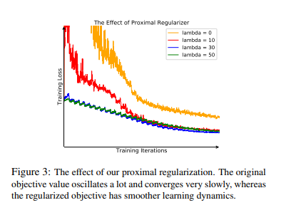
해당 Section에서는 두 가지 물음에 대한 해답을 하고 있다.

1. Sample마다 각각의 Class라고 정의하면, 어떻게 같은 Class와 Similarity Score를 구할 수 있는가?
2. Class당 하나의 Sample만 사용하게 되므로, Learning process가 수렴하기까지 오랜 시간이 걸리거나, 잘 학습이 안 될 것이다.

이러한 문제점을 해결하기 위하여 다음과 같은 Proximal Regularization이 추가되는 식이 Loss로서 사용되었다.

$$J_{NCE}(\theta) = -\mathbb{E}_{P_d}[\text{log}h(i,v_i^{(t-1)} - \lambda \|v_i^{(t)} - v_i^{(t-1)} \|_2^2] - m \cdot \mathbb{E}_{P_n}[\text{log}(1-h(i,v^{'(t-1)}))]$$

• \(t\): Current iteration
• \(V = \{v^{(t-1)}\}\): Memory Bank (Before Iteration Latent Representation)
• \(v_{i}^{(t)} = f_{\theta}(x_i)\): Current Iteration Latent Representation

즉, \(v\)에는 \(\|v\| = 1\)로서 L2 normalization 뿐만 아니라, 이전 Iteration과 비슷하게 Regularizaion을 가하였다. 이러한 결과로서, 수렴 속도를 높이며 Latent Representation을 잘 나타낼 수 있다.

Weighted k-Nearest Neighbor Classifier

Notation

• \((\hat{x})\): Test Image
• \(f_{\theta}(\hat{x})\): Test Image Latent Representation
• \(v_i\): Memory Bank After Training

Non-Parametric Classifier로서 Model을 학습하였기 때문에 Test Image \(\hat{x}\)에 대하여 \(\hat{y}\)는 구할 수 없다. 따라서 해당 논문에서는 \(\text{Model}(f_{\theta}(\hat{x})) = \hat{y}\)에 대한 Model을 Weighte k-Nearest Neighbor Classifier로서 구성하였다.

$$w_c = \sum_{i \in N_k} \alpha_i \cdot 1(c_i = c)$$

• \(N_k\): Top k nearest neighbors
• \(s_i = \text{cos}(v_i, \hat{f})\): Cosine Similarity for Memory Bank After Training & Test Image Latent Representation
• \(\alpha_i = \text{exp}(s_i/\tau)\): wieght
• \(c\): Class
• \(w_c\): Weighted Class

Experiments

많은 Experiment를 진행하였지만, 개인적으로 중요하다고 생각하는 Experiment는 2가지이다.

1. Parametric vs. Non-parametric Softmax

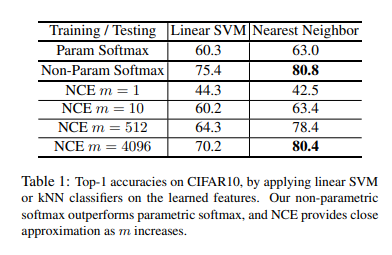
• Number of dataset: 50000
• Number of classes: 10
• Model: ResNet18 (Backbone)
• Dimension of Output Feature: 128

위의 결과를 확인하게 되면, Label정보로서 Classification을 실행시킨 Model인 Param Softmax에 비하여 Non-Param Softmax가 Performance가 높은 것을 확인할 수 있다. 또한, NCE Loss를 사용할때, \(Z \approx Z_i \approx \frac{n}{m} \sum_{k=1}^m \text{exp} (v_{jk}^T f_i / \tau)\)로서 approximation하였지만, m>=4096인 경우 Performance가 거의 비슷한 것을 확인할 수 있었다.

2. Consistency of training and testing objectives

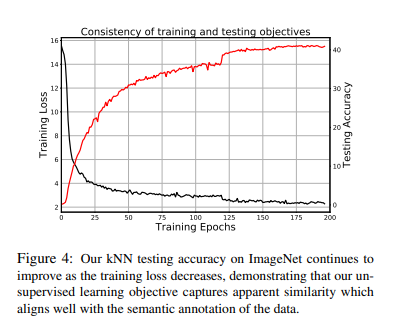
해당 Experiment에 대해서는 논문에 자세히 설명과 잘 정리되어 있어서 그대로 적었습니다.

Unsupervised feature learning is difficult because the training objective is agnostic about the testing objective. A good training objective should be reflected in consistent improvement in the testing performance. We investigate the relation between the training loss and the testing accuracy across iterations. Fig. 4 shows that our testing accuracy continues to improve as training proceeds, with no sign of overfitting. It also suggests that better optimization of the training objective may further improve our testing accuracy

Conclusion

해당 논문에서는 크게 3가지 Main Contribution이 있다고 생각한다.

1. Label정보가 없는 Non-Parametric으로서 학습한 Latent Representation이 Classification에 대한 정보를 잘 나타낼 수 있다는 것이 핵심이였다. 이렇게 학습하는 것은 새로운 Class에 대해서도 잘 예측할 수 있는 Generalization 이 가능하다.
2. 1과 같은 과정에서 Sample의 수가 많아지면, 학습하는데 있어서 Computation Cost가 많이 필요하다. 하지만, Memory Bank와 NCE를 통하여 이러한 Cost를 줄였다.
3. Experiment를 통하여 Training Loss가 줄어듦에 따라서 Classification의 Performance도 증가한다는 것을 알 수 있다.

---

참조: Unsupervised Feature Learning via Non-Parametric Instance Discrimination
참조: zhirongw Github
참조: 2-chae 블로그

코드에 문제가 있거나 궁금한 점이 있으면 wjddyd66@naver.com으로 Mail을 남겨주세요.