Paper15. Contrastive Multiview Coding

Contrastive Multiview Coding

출처: Contrastive Multiview Coding
코드: HobbitLong Github

Abstract

Humans view the world through many sensory channels, e.g., the long-wavelength light channel, viewed by the left eye, or the high-frequency vibrations channel, heard by the right ear. Each view is noisy and incomplete, but important factors, such as physics, geometry, and semantics, tend to be shared between all views (e.g., a “dog” can be seen, heard, and felt). We investigate the classic hypothesis that a powerful representation is one that models view-invariant factors. We study this hypothesis under the framework of multiview contrastive learning, where we learn a representation that aims to maximize mutual information between different views of the same scene but is otherwise compact. Our approach scales to any number of views, and is viewagnostic. We analyze key properties of the approach that make it work, finding that the contrastive loss outperforms a popular alternative based on cross-view prediction, and that the more views we learn from, the better the resulting representation captures underlying scene semantics. Our approach achieves state-of-the-art results on image and video unsupervised learning benchmarks. Code is released at: http://github.com/HobbitLong/CMC/.

Multi-Modality를 사용하는 이유는 다른 논문과 마찬가지로, 서로 다른 Information을 종합하여 좀 더 자세히 Classification이 가능하기 때문이다. 해당 논문에서는 전통적으로 많이 사용하는 cross-view prediction보다 Outperform이 가능한 Contrastive Loss를 적용한 Model을 제시한다.

Introduction

Yet lossless representation might not be what we really want, and indeed it is trivial to achieve – the raw data itself is a lossless representation. What we might instead prefer is to keep the “good” information (signal) and throw away the rest (noise).
For example, a useful representation of images might be a feature space in which it is easy to learn to recognize objects. We therefore evaluate our method by testing if the learned representations transfer well to standard semantic recognition tasks.
Our goal is therefore to learn representations that capture information shared between multiple sensory channels but that are otherwise compact (i.e. discard channel-specific nuisance factors).
Our main contributions are:
• We apply contrastive learning to the multiview setting, attempting to maximize mutual information between representations of different views of the same scene (in particular, between different image channels).
• We extend the framework to learn from more than two views, and show that the quality of the learned representation improves as number of views increase. Ours is the first work to explicitly show the benefits of multiple views on representation quality.
• We conduct controlled experiments to measure the effect of mutual information estimates on representation quality. Our experiments show that the relationship between mutual information and views is a subtle one.
• Our representations rival state of the art on popular benchmarks.
• We demonstrate that the contrastive objective is superior to cross-view prediction.

해당 논문에서 계속해서 던지는 원초적인 질문은 “과연 raw-data를 low-dimension인 latent representation으로서 표현할때 어떤 representation을 좋은 representation이라고 말할 수 있는가?” 이다. 가장 기본적으로 AutoEncoder의 Loss가0이되도록 나타내었을 때, raw-data를 완벽히 reconstruction할 수 있는 latent representation(Encoder output)을 얻을 수 있으 것 이다. 하지만, 이러한 latent representation은 raw-data를 완벽히 압축한 data이기 때문에 필요한 information뿐만 아니라 noise까지 모두 포함하고 있을 것 이다. 해당 논문에서는 Constrative Loss를 활용하여 Embedding하는 법을 제시하고 있다. 아래 그림은 대략적인 Framework를 나타내고 있다.

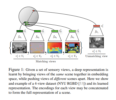
해당 논문에서는 Good bit즉, 좋은 latent representation은 사람이 이해하기 쉽게 Euclidian Distance가 가까우면, 같은 속성을 가지고 있고, 멀리 떨어져있으면 다른 속성을 가지고 있다고 가정하고 있다. 따라서, Multimodality중 같은 Scene은 가깝게 위치하고, 다른 Scene은 멀리 떨어지게 위치하게 하기 위하여 Constrative Loss를 사용하게 된다.

Method

Notation

• \(M\): Number of Modality
• \(V_1, \cdots, V_M\): Data
• \(v_i \text{~} P(V_i)\): random variable representing samples

해당 논문에서는 많이 사용되는 Predictive learning에 비교하여 Constrastive learning의 장점을 설명하고 있다.

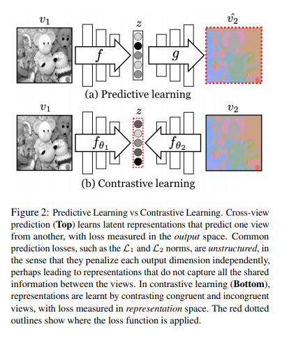
Predictive Learning

먼저 많이 사용되는 Predictive Learning은 Input(\(v_1\))이 Encoder(\(f(\cdot)\))를 거쳐 latent representation(\(z\))으로서 표현된다. 이러한 latent representation은 Decoder(\(g(\cdot)\))을 거쳐 Output(\(\hat{v_2}\))로서 나오게 된다.
결과적인 Loss Function은 \(\hat{v_2} = v_2\)로서 학습되게 된다.

이러한 Loss Function의 단점으로서는 \(p(v_2 | v_1) = \prod_{i} p (v_{2i}|v_1)\)으로서 Complex한 구조를 가지게 되거나, ability가 떨어지게 된다. (많이 사용하는 Multi-modality의 방식이 아니다.)

Contrastive Learning with Two Views

아래 Loss는 Modality가 2인 경우에 Loss Function을 formula로서 나타낸 것 이다.

$$L_{constrast}^{V_1, V_2} = - \mathbb{E}_{\{v_1^1, v_2^1, \cdots v_2^{k+1}\}}[\text{log}\frac{h_{\theta}(\{v_1^1, v_2^1\})}{\sum_{j=1}^{k+1} h_{\theta}(\{v_1^1, v_2^j\})}]$$

• \(k\): Number of Negative Sample
• \(h_{\theta}(\cdot)\): Discriminating function

위의 식을 살펴보면 우리가 많이 보는 Neg Entropy식인 것을 알 수 있다. 또한 K개의 Negative Sample과 1개의 Positive Sample이 Mapping하여 Input Data로서 들어가게 되고, 그 중 Positive Sample일 확률을 높이고, Negative Sample사이의 확률은 낮게 학습되는 것을 살펴볼 수 있다.

즉, \(h_{\theta}(\cdot)\)이 Output단에서 Label을 Prediction하는 Function이면, 기본적으로 많이 사용되는 Classification의 Loss Function형태인 것을 알 수 있다. (단, Input은 Pair로서 Positive, Negative로서 들어가게 된다.)

Implementing the Discriminating Function
Notation

• \(f_{\theta_1}(\cdot), f_{\theta_2}(\cdot)\): Encoder
• \(z_1 = f_{\theta_1}(v_1), z_2 = f_{\theta_2}(v_2)\): Latent Representation
• \(\tau\): Dynamic Range

위와 같이 Notation을 정의하였을때, Discriminatiog Function은 다음과 같이 Cosine Similarity를 활용한 Score로서 나타내었다.

$$h_{\theta}(\{v_1, v_2\}) = \text{exp}(\frac{f_{\theta_1}(v_1) \cdot f_{\theta_2}(v_2)}{\|f_{\theta_1}(v_1)\| \|f_{\theta_2}(v_2)\|}\frac{1}{\tau})$$

최종적인 Loss Function은 다음과 같이 정의할 수 있다. (2 Modality인 경우)

$$L(V_1, V_2) = L_{contrast}^{V_1, V_2} + L_{contrast}^{V_2, V_1}$$

즉, Positive Pair인 경우 Cosine Similarity를 최대화 하고, Negative Pair인 경우 Cosine Similarity를 0으로서 만드는 Contrastive Loss를 Encoder Output(\(z_1, z_2\))에 적용하는 것 이다.

Connecting to mutual information Notation

• \(x \text{~} p(v_1, v_2) = p_d(\cdot)= \{v_1^i, v_2^i\}\): Positive Pair로서 Joint Data Distribution이 존재한다.
• \(y \text{~} p(v_1)p(v_2) = p_n(\cdot) = \{v_1^i, v_2^j\} \text{ .s.t. }i\neq j\): Noise Distribution -> Negative Sample로서 서로 상관없는 Independent한 DataDistribution이다.
• \(S = \{x, y_1, y_2, \cdots, y_k\}\): K개의 Negative Sample있는 경우의 수
• \(h_{\theta}^{*}(\{v_1, v_2\})\): Optimal Score Function

만약, Optimal Probability for the loss p(pos=0|S)는 다음과 같이 표현할 수 있다.

$$p(pos=0|S) = (v_1^0, v_2^0)가 Positive일 확률 * \sum_{j=1}^k (v_1^j, v_2^j)가 Negative일 확률$$

$$= \frac{p_d(v_1^0, v_2^0) \prod_{i=1}^k p_n (v_1^i, v_2^i)}{\sum_{j=1}^k p_d(v_1^j, v_2^h) \prod_{i \neq j} p_n (v_1^i, v_2^i)}$$

$$= \frac{p(v_1^0, v_2^0) \prod_{i=1}^k p (v_1^i) p(v_2^i)}{\sum_{j=1}^k p(v_1^j, v_2^h) \prod_{i \neq j} p(v_1^i) p(v_2^i)}$$

$$= \frac{\frac{p(v_1^0, v_2^0)}{p(v_1^0)p(v_2)^0}}{\sum_{j=0}^k \frac{p(v_1^k, v_2^k)}{p(v_1^k)p(v_2^k)}}$$

$$\approx \frac{p(v_1, v_2)}{p(v_1)p(v_2)}$$

$$(v_1, v_2) \rightarrow (z_1, z_2)$$

$$h^{*}(\{z_1, z_2\}) \approx \frac{p(z_1, z_2)}{p(z_1)p(z_2)}$$

위와같이 변형한 식을 Contrastive Learning with Two Views에 대입하여 Optimal한 \(L_{contrast}^{opt}\)를 구하면 다음과 같다.

$$L_{contrast}^{opt} = - \mathbb{E}_S \text{log}[\frac{h^{*}(\{z_1^0, z_2^0\})}{\sum_{i=0}^k h^{*}(\{z_1^i, z_2^i\})}]$$

$$= -\mathbb{E}_S \text{log}[\frac{\frac{p(z_1^0, z_2^0)}{p(z_1^0)p(z_2^0)}}{\sum_{i=0}^k \frac{p(z_1^i, z_2^i)}{p(z_1^i)p(z_2^i)} }]$$

$$= \mathbb{E}_S \text{log} [1 + \frac{p(z_1^0)p(z_2^0)}{p(z_1^0, z_2^0)} \sum_{i=1}^k \frac{p(z_1^i, z_2^i)}{p(z_1^i) p(z_2^i)}]$$

$$\approx \mathbb{E}_S \text{log} [1 + \frac{p(z_1^0)p(z_2^0)}{p(z_1^0, z_2^0)}k\mathbb{E}_{z_1}[\frac{p(z_1|z_2)}{p(z_1)}]]$$

$$= \mathbb{E}_{S} \text{log} [1+\frac{p(z_1^0)p(z_2^0)}{p(z_1^0, z_2^0)}k]$$

$$\ge \text{log}(k) - \mathbb{E}_{S} \text{log}[\frac{p(z_1^0, z_2^0)}{p(z_1^0)p(z_2^0)}]$$

$$= \text{log}(k) - \mathbb{E}_{(z_1, z_2) \text{~} p_{z_1, z_2}(\cdot)} \text{log}[\frac{p(z_1, z_2)}{p(z_1)p(z_2)}]$$

$$= \text{log}(k) - I(z_1;z_2)$$

$$\therefore I(z_1;z_2) \ge \text{log}(k) - L_{contrast}^{opt}$$

최종적인 식의 결과로서 k(Number of Negative Sample)의 수가 많아질 수록, 좀 더 정확해지는 것을 알 수 있다. 그렇다고 하여서, K를 무작정 큰 수를 선택하게 되면, Optimization Probelm은 어려워지고, \(L_k(V_i, V_j)\)또한 증가되는 것을 알 수 있다.

Contrastive Learning with More than Two Views

2개이상의 Modality가 있을 경우, 크게 2가지 경우로서 나누어서 생각할 수 있다. Figure3은 그 2가지 경우에 대한 예제이다.

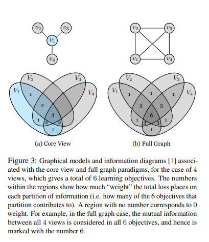
(a) Core View
Core View의 경우에는 \(V_1\)은 다른 모든 Modality와 관계가 있지만, 다른 모든 Modality끼리는 상관이 없다는 가정이다. 이러한 경우에는 다음과 같은 Loss Function을 사용할 수 있다.

$$L_{C} = \sum_{j=2}^M L(V_1, V_j)$$

(b) Full Graph
Full Graph의 경우에는 모든 Modality끼리의 상관관계가 존재한다는 가정이다. 이러한 경우에는 다음과 같은 Loss Function을 사용할 수 있다.

$$L_{F} = \sum_{1 \le i < j \le k} L(V_i, V_j)$$

Implementing the Contrastive Loss

Constrastive Loss를 사용할때 문제점을 현재 논문에서도 얘기하고 있다.
Dataset의 Latent Representation에서 Distance를 기반으로 Loss Function을 구성하기 때문에 Dataset을 Pair로서 잡아야 한다. 현재 논문에서는 Unsupervised Feature Learning via Non-Parametric Instance Discrimination에서 사용한 Memory Bank를 사용하였다고 나와있다. (아직, 읽어보지 않아서 정확한 Implementation은 모르겠습니다.)

참고: Paper11. SoftTriple에서도 위와같은 문제 때문에, Class별 K개의 Group으로서 Clustering하는 Loss를 사용하여 문제를 해결하였다.

Experiments

현재 논문에서 크게 살펴봐야할 실험결과는 2가지 이다.

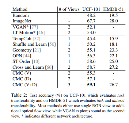
Modality를 증가시킴에 따라서 Performance가 증가하였고, 다른 Classification Model보다 성능이 좋다.

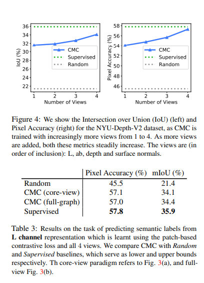
위의 결과가 가장 흥미로운 결과였다. 중요한것은 End-to-End를 기반으로 학습된 Supervised U-Net에 비하여, Modality가 충분히 많다면, CMC는 Latent Representation와 비슷한 효과를 낼 수 있다는 것 이다. 또한, Core-view와 Full-Graph의 성능차이가 거의 나지 않았다.

Conclusion

해당 논문에서는 Feature Embedding상에서 Multimodality끼리도, 상관이 있으면 가까운 Distance에, 상관이 없으면 먼 Distance에 배치하기 위하여 Constrastive Loss를 적용한 Model이다. 해당 Model은 간단한 생각인 Modality에 상관없이 Positive Sample간에 Joint Distribution을 최대화 하고, Negative Sample간에는 Noise로서 생각하여 Loss를 구축하였다. 또한, Core View와 Full Graph라는 Multimodality에서 큰 2가지 상황에 대하여 모두 적용할 수 있다는 것이 큰 장점이다.

Appendix - Open Review

해당 논문에서 가지는 의문점이 Open Review에 동일하게 나와있는 부분이 있었다.

1. The core concept, or at least one of the core concepts, in multi-view learning is the conditional independence.
   Normally, the underlying assumption in multi-view learning is that, given the class label, the samples from multiple views are conditionally independent from each other. Therefore, the goal is to learn distinctive representations from different data sources/disjoint populations, so then after learning, the ensemble of them is able to capture a set of diverse aspects of the data. A “side-effect” of learning from multiple views is that individual views indeed get improved by learning from others. Meanwhile, self-supervised learning is the case when the input data to the designed learning system is also the target of the system.
2. My main concern of this paper is the novelty, however, the empirical results are strong.
   The paper mainly presented a simple yet effective method for self-supervised learning from two views, and the generalisation is a sum over all possible combinations of two views. The method itself has already been proposed many years ago as mentioned in the related work section in the paper, and the generalisation was also described in prior work, which makes me doubt the novelty of the paper.

1의 의문은 Paper를 가지고 있던 의문이다. 서로 다른 Modality간에 Independent가 보장되어야 Loss Function의 식이 유도될 수 있다. 하지만, 이러한 Independent가 보장된다면, 충분히 Ensemble로서도 효과를 낼 수 있다는 reviewer의 입장이였다.

1. 기존에 많이 사용되던 Loss를 정리한 것이라고 표현하고 있다. 개인적으로는 Contrastive Learning with More than Two Views로서 크게 2가지로 나눈 것은 매우 참신하였으나, 나머지는 기존에 많이 사용하는 방법인 것에 대하여 동의한다.

Pytorch Code (HobbitLong Github)

특별한 것이 없어서 따로 정리하지 않았습니다.

---

참조: Contrastive Multiview Coding
참조: HobbitLong Github

코드에 문제가 있거나 궁금한 점이 있으면 wjddyd66@naver.com으로 Mail을 남겨주세요.