Paper17. FaceNet: A Unified Embedding for Face Recognition and Clustering

FaceNet: A Unified Embedding for Face Recognition and Clustering

출처: FaceNet: A Unified Embedding for Face Recognition and Clustering

Abstract

Despite significant recent advances in the field of face recognition [10, 14, 15, 17], implementing face verification and recognition efficiently at scale presents serious challenges to current approaches. In this paper we present a system, called FaceNet, that directly learns a mapping from face images to a compact Euclidean space where distances directly correspond to a measure of face similarity. Once this space has been produced, tasks such as face recognition, verification and clustering can be easily implemented using standard techniques with FaceNet embeddings as feature vectors.
Our method uses a deep convolutional network trained to directly optimize the embedding itself, rather than an intermediate bottleneck layer as in previous deep learning approaches. To train, we use triplets of roughly aligned matching / non-matching face patches generated using a novel online triplet mining method. The benefit of our approach is much greater representational efficiency: we achieve state-of-the-art face recognition performance using only 128-bytes per face.
On the widely used Labeled Faces in the Wild (LFW) dataset, our system achieves a new record accuracy of 99.63%. On YouTube Faces DB it achieves 95.12%. Our system cuts the error rate in comparison to the best published result [15] by 30% on both datasets.
We also introduce the concept of harmonic embeddings, and a harmonic triplet loss, which describe different versions of face embeddings (produced by different networks) that are compatible to each other and allow for direct comparison between each other.

해당 논문은 Triplet Loss를 최초는 아니지만, Application으로서 처음으로 효과적이라는 것을 밝힌 논문이다. 해당 논문에서는 FaceNet을 제시하고 있다. 이 Model은 Face Recognization에서 SOTA(State-Of-The-Art) Performance를 보여주고 있다. 주요한 점은 Tripletloss를 사용하여, Latent Representation상에서 Euclidian Distance기반으로서 학습한다는 것 이다.

Introduction

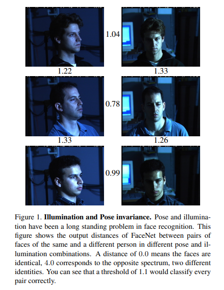
위의 사진은 Triplet Loss로서 학습한 Model의 장점을 설명하고 잇다. 각각의 오른쪽과 왼쪽의 사진은 같은 Sample이나, Position이 다르다. 위 아래로는 다른 Sample이다.
Triplet Loss로서 학습한 FaceNet으로서는 Position이 달라도 같은 Sample이면 Distance가 가깝고, 다른 Sample이면 Distance가 먼 것을 확인할 수 있다.

이러한 결과를 얻기 위하여 Triplet Loss를 사용한 이유를 해당 논문에서는 다음과 같이 언급하고 있다.

Previous face recognition approaches based on deep networks use a classification layer [15, 17] trained over a set of known face identities and then take an intermediate bottleneck layer as a representation used to generalize recognition beyond the set of identities used in training.
The downsides of this approach are its indirectness and its inefficiency: one has to hope that the bottleneck representation generalizes well to new faces; and by using a bottleneck layer the representation size per face is usually very large (1000s of dimensions).
Some recent work [15] has reduced this dimensionality using PCA, but this is a linear transformation that can be easily learnt in one layer of the network.

Latent Representation에서 Distance기반으로 학습하는 이유에 대하여 설명하고 있다. 이전까지의 Traditional한 CNN의 기반의 Model은 Classifier로서 학습을 하게 되었다. 이러한 결과로서 새로운 Dataset에 대해서는 Overfitting을 발생할 수 있는 요소가 많다. 이러한 문제를 해결하기 위하여 PCA와 같은 Dimension Reduction방법을 사용하게 되면, Linear한 Transformation만 가능하다는 단점을 발생시킬 수 있다. 해당 논문에서는 이러한 Indirectness하고 Inefficiency한 단점을 해결하기 위하여 Triplet Loss를 사용하였다고 한다.

참초: Why CNN is indirectness & inefficiency -> Not well generalization (해당 section은 개인적인 생각입니다.)
해당 논문에는 자세히 나와 있지 않다. 왜 CNN + Classifier로서 학습하는 것은 Indirectness하고 Inefficiency하여 generalization이 안되는 것 일까? 개인적인 생각으로는 Latent Representation -> Classifier로서 갈때 Feature의 중요도를 판단하기 때문이다.
예를 들어 Image(224 x 224)를 CNN의 Bottleneck Output으로서 128 Dimension으로서 Mapping하였다고 생각해보자. 이러한 Output은 Image를 구별할 수 있는 큰 특징들을 포함하고 있을 것이다. 예를들어, 눈, 코, 입 과 같은 특징을 배운다고 생각하자. 이러한 Output을 구별하기 위하여 Classifier를 학습하게 되면 어쩔 수 없이 눈, 코, 입 중 가장 두드러지는 특징인 “눈”에 집중하여 판별할 수 밖에 없다고 생각한다. 하지만, Latent Representation상에서 Distance로서 판단하게 되면, 눈, 코, 입을 모두 고려하여 Classification이 가능할 것 이다.
이러한 이유로서 Latent Representation에서 Distance기반으로서 학습하는 Contrastive Learning의 Model들은 Dataset이 Pair로서 잡혀 많아지게 되는 단점이 생기지만, 적은 Dataset에서 효과적인 것 같다.

Method

Notation

• \(f(\cdot)\): CNN Embedding Model(Inception)
• \(x\): Input
• \(\mathbb{R}^d\): feature sapce (\(f(x) \in \mathbb{R}^d\))
• \(\tau \in \mathbb{R}^N\): All possible Triplets in the training set
• \(x_i^a\): i-th sample & Anchor
• \(x_i^p, x_i^n\): i-th sample & Posive, Negative
• \(\alpha\): margin

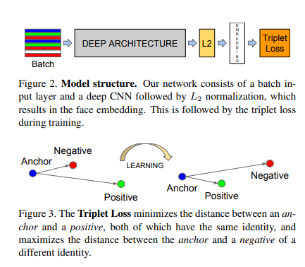
위의 Figure를 살펴보게 되면, \(x \rightarrow \text{Deep Architecture} \rightarrow L2 \rightarrow \text{Embedding}\)이 \(f(x)\)인 것을 확인할 수 있다. 즉, \(\|f(x)\|_2 = 1\)이다.

또한, Triplet Loss를 살펴보게 되면, 기준이 되는 Anchor를 기준으로서 같은 Label은 가까운 거리에 위치하게 학습하고 다른 Label은 먼 거리에 학습시키는 방법인 것을 살펴 볼 수 있다. 각각의 Anchor, Anchor와 Positive & Negative에 대해서는 위의 Notation과 같이 나타낸다.

TripletLoss

$$\text{TripletLoss} = \sum_{i}^N [\|f(x_i^a) - f(x_i^p)\|_2^2 - \| f(x_i^a) - f(x_i^n)\|_2^2 +\alpha]_{+}$$

$$\forall(f(x_i^a), f(x_i^p), f(x_i^n)) \in \tau$$

위의 식을 살펴보면 간단하다. Anchor를 기준으로 Positive와의 거리가 Negative의 거리보다 Margin(\(\alpha\))이상으로 가깝게 학습하는 것 이다.
즉, Anchor를 기준으로 Negative Sample과의 거리는 Posivie Sample과의 거리 + Margin(\(\alpha\))이상으로서 학습하게 되므로서 같은 Label끼리는 가까운 Distance상에 위치하게 되고, 다른 Label끼리는 상대적으로 먼 Distance에 위치하게 된다.

Triplet Selection
Contrastive Learning에서 항상 문제가 되는 것 이다. Dataset을 Pair로서 잡게 되면 \(\tau\)에서 가능한 수는 \(N^3\)으로서 매우 커지게 된다.

이러한 \(\tau\)안에서 선택해야 하는 sample은 \(\text{argmax}_{x_i^p}\|f(x_i^a) - f(x_i^p)\|_2^2\)(Hard Positive), \(\text{argmin}_{x_i^n}f(x_i^a) - f(x_i^n)\|_2^2\)(Hard Negative)인 것을 알 수 있다.
즉, Anchor를 기준으로 멀리 떨어져있는 Positive를 Anchor와 가깝게 위치시키고, Anchor를 기준으로 가까운 Negative를 Anchor와 멀리 떨어지게 학습시킬 수 있는 Hard Positive와 Hard Negative를 선택하는 것이 Model을 Training하는 과정에서 Converge되는 속도가 빠를 것이라고 예상할 수 있다.

하지만, 모든 Train Sample에서 매번 이러한 계산을 하는 것은 어려운 것을 알 수 있다. 해당 논문에서는 이러한 문제를 해결하기 위한 Sampling방법을 다음과 같이 적어두었다.

To have a meaningful representation of the anchor positive distances, it needs to be ensured that a minimal number of exemplars of any one identity is present in each mini-batch.
Instead of picking the hardest positive, we use all anchorpositive pairs in a mini-batch while still selecting the hard negatives. We don’t have a side-by-side comparison of hard anchor-positive pairs versus all anchor-positive pairs within a mini-batch, but we found in practice that the all anchorpositive method was more stable and converged slightly faster at the beginning of training.
Selecting the hardest negatives can in practice lead to bad local minima early on in training, specifically it can result in a collapsed model (i.e. f(x) = 0).

Sampling방법에 대하여 Triplet Loss에서 중요한 몇가지에 대해서 적어두었다.

1. 모든 Training Set에 대하여 Hard Positive, Hard Negative를 선택하는 것은 불가능 하므로, 각각의 Batch단위에서 Sampling을 실시하였다.
2. 모든 Positive Sample을 사용하고, Hard Negative를 사용하는 것이, Hard Positive를 선택하는 것보다 Stable하게 수렴하였다.
3. 학습 초기에는 Hard Negative를 선택하는 것은 Local Minimun을 유발할 수 있다.

중요한 실험결과라고 생각하고 있다.
2의 경우에는 만약, Outlier인 Anchor를 선택하게 되면, 모든 Positive Sample이 Hard Negative로서 선택되게 되고, 따라서 학습은 안좋은 방향으로 이루워 질 수 있다. 따라서 Stable하게 학습이 될 수 없다.
3의 경우도 마찬가지이다. 학습초기에 Hard Negative를 선택한다는 것은 Outlier이거나, Label이 잘못선정된 Sample일 확률이 높다. 따라서 이러한 Sample만을 선택하여 학습하는 것은 Local Minimum을 유발할 수 있다.

Experiments and Evaluation

Evaluation

• \(D(x_i, x_j)\): squared \(L_2\) Distance
• \(P_{\text{same}}\): Same identity
• \(P_{\text{same}}\): Different identity
• \(\text{TA}(d) = {(i,j) \in P_{\text{same}}, \text{ with } D(x_i, x_j) \le d}\)
• \(\text{FA}(d) = {(i,j) \in P_{\text{diff}}, \text{ with } D(x_i, x_j) \le d}\)
• \(\text{VAL}(d) = \frac{|TA(d)|}{|P_{\text{same}}|}\): 같은 Identity에 대해서 Classification또한 같은 Identity라고 평가한 것 이다. (True Classification)
• \(\text{FAR}(d) = \frac{|FA(d)|}{|P_{\text{diff}}|}\): 다른 Identity에 대해서 CLassification은 같은 Identity라고 평가한 것 이다. (False Classification)

Evaludation의 평가 지표는 크게 2가지 \(\text{VAL}(d)\), \(\text{FAR}(d)\)이다.

Experiments
주요하게 살펴본 Experiment결과는 2개이다.

Sensitivity to Image Quality

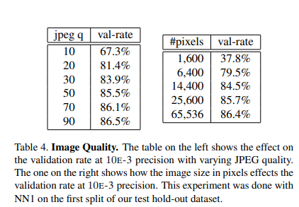
위의 결과는 Robust하다는 것을 의미하고 있다. Model을 Training하는 Input Data는 220 x 220으로서 학습하였으나, Pixels가 매우 작거나 Image Quality가 매우 낮은 jpeg q = 10을 제외하고는 어느정도 성능이 유지되었다. 즉, 어떠한 Input에 대해서도 다른 Model에 비하여 Robust하다는 것을 알 수 있다.

Embedding Dimensionality

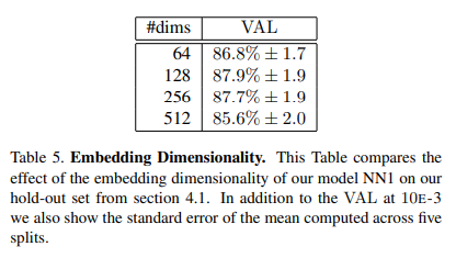
위의 결과로서 의미하는 바는 “Dimension이 작아도 충분히 큰 Dimension과 비슷한 효과를 낼 수 있다. 하지만, Dimension이 크면 클 수록 훈련시간이 오래 걸린다.” 는 결론을 얻을 수 있다. 즉, 매우 작은 Dimension만 아니면, Model의 Performance는 어느정도 보장되므로, 작은 Dimension으로 이루워지는 Model로서 용량을 줄여서 Mobile Device에서도 가능할 것이라는 결론을 내고 있다.

Conclustion

해당논문은 TripletLoss를 초창기에 사용한 논문으로서 새로운 Insight를 얻을 수 있는 것을 별로 없었다. 하지만, TripletLoss에 대해서 자세히 설명하고, 특히 Sampling에 대한 자세한 내용은 많은 도움이 되었다.

Appendix

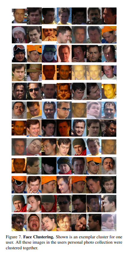
위의 사진은 해당 Model에서 잘못 Clustering한 결과를 보여주고 있다. 솔직히, 사람인 내가 보아도 같은 인물로서 보인다.

---

참조: FaceNet: A Unified Embedding for Face Recognition and Clustering

코드에 문제가 있거나 궁금한 점이 있으면 wjddyd66@naver.com으로 Mail을 남겨주세요.