
Paper03. Extreme Learning Machine
ExtrmeLearningMachine
Extreme Learning Machine for Regression and Multiclass Classification (https://ieeexplore.ieee.org/stamp/stamp.jsp?tp=&arnumber=6035797)
Representational Learning with Extreme Learning Machine for Big Data(https://pdfs.semanticscholar.org/8df9/c71f09eb0dabf5adf17bee0f6b36190b52b2.pdf)
Abstract
This paper shows that both LS-SVM and PSVM can be simplified further and a unified learning framework of LS-SVM, PSVM, and other regularization algorithms referred to extreme learning machine (ELM) can be built.
ELM works for the “generalized” single-hidden-layer feedforward networks (SLFNs), but the hidden layer (or called featuremapping) in ELM need not be tuned.
Such SLFNs include but are not limited to SVM, polynomial network, and the conventional feedforward neural networks.
Abstract를 살펴보게 되면, ELM은 Single Hidden Layer Feedforward Network에 대하여 Generalized된 형태로 Work할 수 있다고 설명하고 있다.
이러한 ELM을 Optimization하기 위하여 SVM의 식을 사용하여 증명하였고, 중요한 것은 Hidden Layer로서 Mapping하기 위하여 Weight, Bias를 학습하는 것이 아니라 Hidden Layer에서 Target Space로 Mapping하는 Weight에 대하여 학습하여 이루워 진다는 것 이다.
ExtrmeLearningMachine을 살펴보면 다음과 같은 형태를 띄고 있다.
Background(SVM)
Decision Boundary(Hyperplane): \(f(x) = wx + b = a\)라고 가정하면, a>0 => Positive, a<0 => Negative로서 Prediction가능하다.(Label이 Binary인 경우)
Maximizing the Margin
- \(x_p\): Hyperplane위의 Point
- \(f(x) = wx+b = a \text{ or } -a\): Support Vector
- \(w\): Hyperplane의 접선 Vector
- \(r\): Hyperplane의 에서 Support Vector 까지의 거리
위와 같이 가정하였을 경우 다음과 같이 x를 정의할 수 있다.
$$x=x_p + r\frac{w}{||w||}$$
즉, 임의의 한 Point는 Hyperplane위의 Point를 기준으로 방향은 w, 크기는 r인 Vector로서 표현할 수 있는 것 이다.
위의 식을 활용하면 다음과 같다.
$$f(x) = w(x_p + r \frac{w}{||w||})+b = r||w|| (\because f(x_p) = wx_p+b = 0)$$
$$\therefore r = \frac{f(x)}{||w||} \rightarrow \text{margin} = \frac{2a}{||w||}$$
위에서 Support Vector의 값을 a라고 하였으므로 다음과 같이 표현할 수 있다.
$$max_{w,b}2r = \frac{2a}{||w||}$$
$$s.t(wx_j+b)y_j \ge a$$
위의 식에서 a는 임의의 상수이므로 a=1이라 가정하면 최종적인 Maximizing the Margin은 다음과 같이 나타낼 수 있다.
\(min_{w,b}||w||\) \(s.t.(wx_j+b)y_j \ge 1\)
Error Handling in SVM
Decision Boundary밖에 Label이 다른 Point가 있는경우 위의 Formular로서는 Optimization이 불가능 하므로, 이러한 Point에 대하여 Penalty를 Hinge Loss로서 구현하면 식을 다음과 같이 정의할 수 있다.
$$min_{w,b}||w||+C\sum_{j}\xi_j$$
$$s.t(wx_j+b)y_j \ge 1-\xi_j$$
$$\xi_j \ge 0$$
$$\text{EX) } \xi_j =(1-(wx_j+b)y_j)_{+}$$
Proposed Constrained Optimization Based ELM
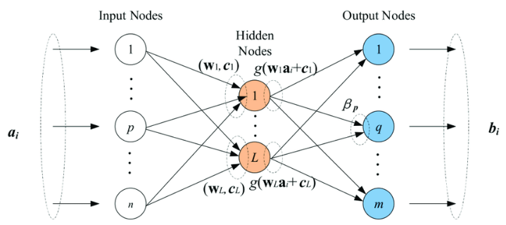
ELM for generalized SLFNS
$$f_L(x) = \sum_{i=1}^L \beta_i h_i(x) = h(x)\beta$$
- \(\beta = [\beta_1,\beta_2, ..., \beta_L]^T\): The vector of the output weights between the hidden layer of L nodes
- \(h(x) = [h_1(x),h_2(x), ..., h_L(x)]^T\): The output vector of the hidden layer with respect to the input X. ex) ANN => \(\sigma(wx+b)\)
위와 같이 정의하였을 때, Label이 -1 or 1 의 Binary Label로서 \(f_L(x)\)가 Classification Model이라고 가정하여 Prediction의 값은 \(f_L(x) = sing(h(x)\beta)\)로서 표현할 수 있을 것 이다.
즉, ELM은 Input X를 어떠한 Hidden Layer인 H Space에 Mapping하였을 때, 이러한 Hidden Space에서 Target Space로서 Mapping하는 \(\beta\)를 잘 학습하자는 것이 목표가 된다. 또한, Generalize한 Model이라고 말할 수 있는것은, Hidden Layer는 상관없기 때문이다.
위와 같은 수식을 Optimize하는 식은 다음과 같이 나타낼 수 있다.
Optimize
$\text{Minimize: }||H\beta -T||^2 \text{ and }||\beta|| \text{ , T: Label}$
- Term1: \(||H\beta -T||^2\): Prediction값과 Label의 값을 Minimize한다.
- Term2: \(||\beta||\): Maximize the distance of the separating margins of the two different classes in the ELM feature Space
위의 식을 살펴보게 되면, SVM을 Optimize하는 식(\(min_{w,b}||w||+C\sum_{j}\xi_j\))같다는 것을 알 수 있다.
위의 식을 각각의 Prediction마다 Error로서 바꾸고 Generalization Form으로서 바꾸면 다음과 같이 나타낼 수 있다.
$$\text{Minimize: }L = \frac{1}{2} ||\beta||^2 + C \frac{1}{2}\sum_{i=1}^N \xi_i^2$$
$$\text{Subject to: }h(x_i)\beta = t_i-\xi_i \text{, i=1,...,N}$$
위의 식을 Optimize하기 위하여 KKT Condition으로서 나타내면 다음과 같다. (or FISTA Algorithm으로서 Optimization한 Paper도 존재)
KKT Condition
$$L = \frac{1}{2} ||\beta||^2 + C \frac{1}{2}\sum_{i=1}^N \xi_i^2 - \sum_{i=1}^N \alpha_i(h(x_i)\beta = t_i-\xi_i)$$
$$\alpha_i\text{: Lagrange multiplier corresponds to the ith trainning sample}$$
KKT Optimality Conditions
- \(\frac{\partial L}{\partial \beta} = 0 \rightarrow \sum_{i=1}^N \alpha_i h(x_i)^T = H^T \alpha\)
- \(\frac{\partial L}{\partial \xi_i} = 0 \rightarrow \alpha_i = C \xi_i\)
- \(\frac{\partial L}{\partial \alpha_i} = 0 \rightarrow h(x_i)\beta-t_i+\xi_i=0\)
Optimal \(\beta\)
위의 KKT Optimality Condition을 만족하는 Optimal \(\beta\)는 다음과 같이 구할 수 있다.
$$h(x_i)\beta + \xi_i = t_i$$
$$h(x_i)\beta + \frac{1}{C}\alpha_i = t_i (\because\xi_i = \frac{\alpha_i}{C})$$
$$h(x_i)H^T \alpha + \frac{1}{C}\alpha_i = t_i (\because \beta = H^T\alpha)$$
$$\sum_{i=1}^N h(x_i)H^T \alpha + \frac{1}{C}\alpha_i = \sum_{i=1}^N t_i$$
$$(\frac{I}{C}+HH^T)\alpha = T$$
$$\alpha = (\frac{I}{C}+HH^T)^{-1}T$$
$$\beta = H^T(\frac{I}{C}+HH^T)^{-1}T (\because \beta = H^T\alpha)$$
Result of ELM
Abstract에서 설명한 ELM works for the “generalized” single-hidden-layer feedforward networks (SLFNs), but the hidden layer (or called featuremapping) in ELM need not be tuned에 대한 내용을 다시한번 생각하면 다음과 같다.
ELM은 Input Data를 Hidden Layer에 Mapping하는 것은 Tuning하지 않고, 이러한 Hidden Layer에서 Target Layer에 Mapping하는 과정에 대해서만 고려한다.
이로인하여 어떠한 Hidden Layer에서 Work하는 Solution이 될 수 있으며, Normal Equation으로서 Hidden Layer => Target Space로 Mapping or Classification에 대해서도 Optimal한 Solution이 있다는 것을 증명하였다.
Paper에서는 대표적인 Hidden Layer에 대하여 다음과 같이 정의하였다.
$$h(x) = [G(a_1,b_1,x),...,G(a_L,b_L,x)]$$
- Sigmoid Function: \(G(a,b,x) = \frac{1}{1+exp(-(ax+b))}\)
- Hard-limit Function: \(G(a,b,x) = \begin{cases} 1, & \mbox{if }ax-b \ge 0 \\ 0, & \mbox{otherwise.} \end{cases}\)
- Gaussian Function: \(G(a,b,x) = exp(-b||x-a||^2)\)
- Multiquadric Function: \(G(a,b,x) = (||x-a||^2+b^2)^{1/2}\)
ELM은 Global Optimum을 가지고, 어떠한 Hidden Layer와 상관없이 잘 작동하는 Generalize한 Model이나, 결국 Normal Equation으로서 모든 Matrix연산을 수행해야 하므로, OOM에 문제가 많아서, 특정 Task에서만 사용한다.(Data가 작고, Feature가 작은 Task)
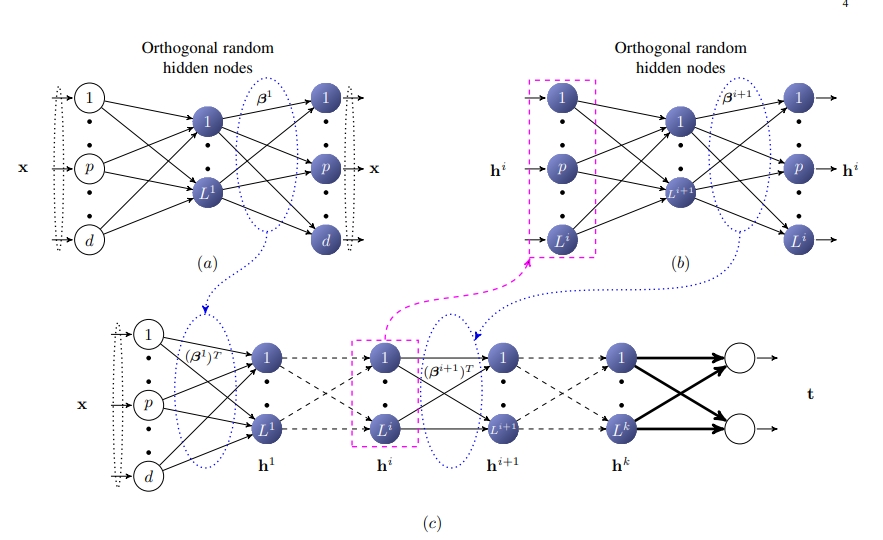
Multi Layer Extrme Learning Machine
Multi Layer Extreme Learning Machine은 single-hidden-layer feedforward networks (SLFNs)에 Generalization된 Extreme Learning Machine을 여러 Layer로서 구성하는 것 이다.
각각의 Layer는 AutoEncoder구조로서 쌓이게 된다.
Extreme Learning Machine AutoEncoder를 살펴보면 아래와 같다.
Extreme Learning Machine Auto Encoder
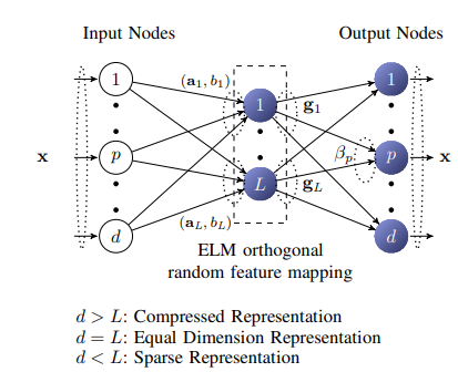
- \(h=g(ax+b) \text{ ,g: Activation Function}\)
- \(a^T a = I, b^T b = 1\)
- \(a = [a_1, a_2, a_3, ..., a_L]\): Orthogonal Random Weight
- \(b\): Orthogonal random Bias
위에서 Weight(a), Bias(b)를 Orthogonal로서 Initialization하는 이유는 Random하게 Initialization하되 좀 더 Generalization이 잘 되는 Model로서 만들기 위한 과정이다.
또한 g는 Activation Function으로서 Linear한 Structure or Non-Linear한 Structure로서 구성할 수 있다.
이러한 Extreme Learning Machine Auto Encoder로서 Multi Layer Extreme Machine을 구성하면 다음과 같다.
Linear ML-ELM(Muiti Layer Extreme Machine) Representational Learning with Extreme Learning Machine for Big Data Paper를 살펴보면 Linear ML-ELM을 다음과 같이 구성하였다.
- \(h=g(ax+b) \text{ ,g: Orthogonal Random Feature Mapping}\)
- \(a^T a = I, b^T b = 1\)
- \(a = [a_1, a_2, a_3, ..., a_L]\): Orthogonal Random Weight
- \(b\): Orthogonal random Bias
위에식을 살펴보게 되면, Activation Function으로서 Orthogonal Random Feature Mapping을 사용하였다.
즉 h=g(ax+b)가 Orthogonal Matrix이므로 다음과 같은 식이 성립한다.
$$\beta = (\frac{I}{C}+HH^T)^{-1}H^TX = H^{-1}X \text{, }(\because HH^T = I) $$
$$\beta^{T} \beta =I \text{, (if X = Orthogonal Matrix)}$$
즉, 첫 Input으로 들어오는 X는 Orthogonal Matrix가 아니므로, g로서 Orthogonal Random Feature Mapping을 한 뒤부터는 Input이 Orthogonal Matrix이므로 위의 식이 성립하게 된다.
단순히 Activation Function이 Orthogonal Random Feature Mapping이므로, Linear한 Activation Function을 적용한 것이라고 생각할 수 있다.**
Non-Linear ML-ELM(Muiti Layer Extreme Machine)
위의 Linear ML-ELM을 생각해보면, Hidden Space => Orthogonal Matrix & X => Orthogonal Matrix이므로, \(\beta^{-1} = \beta^T\)가 성립하여 \(h = \beta^T X\)가 성립하였다.
하지만, Activation Function을 우리가 주로사용하는 Sigmoid Funcitno을 사용하게 되면, X => Orthogoanl, W => Orthogonal, B => Orthogonal이여도, \(\sigma(WX+B)\)는 Orthogonal Matrix가 되지 않는다.
따라서 \(h = \beta^{*}X \text{, }\beta^{*}\text{ = pseudoinverse}\)로서 Extreme Learning Machine Auto Encoder를 사용하여 Layer를 쌓아야 한다.
ExtrmeLearningMachine Code
위에서 언급한 ExtremeLearningMachine을 FISTA Algorithm(L1 Regularization)으로서 구성하면 다음과 같다.
ExtremeLearningMachine
1
2
3
4
5
6
7
8
9
10
11
12
13
14
15
16
17
18
19
20
21
22
23
24
25
26
27
28
29
30
31
32
33
34
35
36
37
38
39
40
41
42
43
44
45
46
47
48
49
50
51
52
53
54
55
56
57
58
59
60
61
62
63
64
65
66
67
68
69
70
71
72
73
74
75
76
77
78
79
80
81
82
83
84
85
86
87
88
89
90
91
92
93
94
95
96
97
98
99
100
101
102
103
104
105
106
107
108
109
110
111
112
113
114
115
116
117
118
119
120
121
122
123
124
125
126
127
128
129
130
131
132
133
134
135
136
137
138
139
import numpy as np
from sklearn.base import ClassifierMixin, BaseEstimator
from scipy import linalg
from math import sqrt
from sklearn.metrics.pairwise import rbf_kernel

# Extreme Learning Machine
class ELM(BaseEstimator, ClassifierMixin):
    # Input -> Hidden Layer -> Output
    def __init__(self, hid_num, linear, ae, activation='sigmoid'):
        # hid_num (int): number of hidden neurons
        self.hid_num = hid_num
        # linear (bool): Linear ELM AutoEncoder or Non Linear AutoEncoder
        self.linear = linear
        # ae (bool): ELM AutoEncoder or ELM Classifier
        self.ae = ae
        # Activation Function: Sigmoid or ReLu or Tanh
        self.activation = activation

    # Sigmoid Function with Clip Data
    def _sigmoid(self, x):
        # Sigmoid Function with Clip
        sigmoid_range = 34.538776394910684
        x = np.clip(x, -sigmoid_range, sigmoid_range)
        return 1 / (1 + np.exp(-1 * x))

    # ReLU Function
    def _relu(self, x):
        return x * (x > 0)

    # Tanh Function with Clip Data
    def _tanh(self, x):
        return 2*self._sigmoid(2*x)-1

    # For Last Layer => Classification => Multiclass
    def _ltov(self, n, label):
        # Trasform label scalar to vecto
        return [-1 if i != label else 1 for i in range(1, n + 1)]

    # Weight Initialization => Unit Orthogonal Vector, Unit Vector
    def weight_initialization(self, X):
        # Weight Initialization => Orthogonal Matrix, Scaling = 1
        u, s, vh = np.linalg.svd(np.random.randn(self.hid_num, X.shape[1]), full_matrices=False)
        W = np.dot(u, vh)

        # Bias Initialization => Unit Vector
        b = np.random.uniform(-1., 1., (1, self.hid_num))
        # find inverse weight matrix
        length = np.linalg.norm(b)
        b = b / length

        return W, b

    # For Fista Algorithm
    def _soft_thresh(self, x, l):
        return np.sign(x) * np.maximum(np.abs(x) - l, 0.)

    # Fista algorithm for L1 regularization
    def fista(self, X, Y, l, maxit):
        if not self.ae:
            x = np.zeros(X.shape[1])
        else:
            x = np.zeros((X.shape[1], Y.shape[1]))
        t = 1
        z = x.copy()
        L = np.maximum(linalg.norm(X) ** 2, 1e-4)

        for _ in range(maxit):
            xold = x.copy()
            z = z + X.T.dot(Y - X.dot(z)) / L
            x = self._soft_thresh(z, l / L)
            t0 = t
            t = (1. + sqrt(1. + 4. * t ** 2)) / 2.
            z = x + ((t0 - 1.) / t) * (x - xold)
        return x

    # Training => Find β
    def fit(self, X, y, iteration=1000, l=0.01):

        # For One Single Layer AutoEncoder
        if not self.ae:
            # number of class, number of output neuron
            self.out_num = max(y)

            if self.out_num != 1:
                y = np.array([self._ltov(self.out_num, _y) for _y in y])

        # Orthogonal Unit Matrix
        self.W, self.b = self.weight_initialization(X)

        # Linear ELM Auto Encoder
        # H = Orthogonal Matrix Mapping
        if self.linear:
            self.H = np.dot(X, self.W.T) + self.b
            u, s, vh = np.linalg.svd(self.H, full_matrices=False)
            self.H = np.dot(u, vh)

        # Non Linear EML Auto Encoder
        # H = Sigmoid(wx + b) or ReLU(wx + b) or Tanh(wx + b)
        else:
            # Activation Function => Sigmoid Function
            if self.activation == 'sigmoid':
                self.H = self._sigmoid(np.dot(self.W, X.T) + self.b.T).T

            # Activation Function => ReLU Function
            elif self.activation == 'relu':
                self.H = self._relu(np.dot(self.W, X.T) + self.b.T).T

            # Activation Function => Tanh Function
            else:
                self.H = self._tanh(np.dot(self.W, X.T) + self.b.T).T

        # Single Layer ELM or For ELM AutoEncoder
        if not self.ae:
            self.beta = self.fista(self.H, y, l, iteration)

        else:
            self.beta = self.fista(self.H, X, l, iteration)

        return self

    # if One Single Layer ELM => Predict
    def predict(self, X):

        if self.linear:
            H = np.dot(X, self.W.T) + self.b
            u, s, vh = np.linalg.svd(H, full_matrices=False)
            H = np.dot(u, vh)
            y = np.dot(H, self.beta)

        else:
            H = self._sigmoid(np.dot(self.W, X.T) + self.b.T)
            y = np.dot(H.T, self.beta)

        if self.ae == True:
            return y

        else:
            return np.sign(y)
Kernel ExtremeLearningMachine
ExtremeLearningMachine에 Gaussian Kernel(rbf kernel)을 사용하여 구성하면 다음과 같다. (Classifier로 사용 가능)
1
2
3
4
5
6
7
8
9
10
11
12
13
14
15
16
17
18
19
20
21
22
23
24
25
26
27
28
29
30
31
32
33
34
35
36
37
38
39
40
41
42
43
44
45
# Kernel Extreme Learning Machine
class KELM(BaseEstimator, ClassifierMixin):
    # Input -> Hidden Layer -> Output
    def __init__(self):
        # Kernel
        self.kernel = None
        # l (float) : regularization term
        self.l = 0.001

    def fit(self, X, y, l=0.001):
        self.X = X
        self.y = y

        self.out_num = max(y)

        # Train Kernel and Hidden Space
        self.kernel = rbf_kernel(self.X, self.X)
        self._H = np.linalg.inv(np.diag(np.tile(l, self.kernel.shape[0])) + self.kernel) @ y

        return self

    def predict(self, test_X):
        # Predict by rbf kernel
        y = np.ones((self.X.shape[0], test_X.shape[0]))

        for i in range(self.X.shape[0]):
            y[i] = np.array(rbf_kernel(test_X, self.X[i].reshape(1, -1))).squeeze()

        y = np.dot(y.T, self._H)

        if self.out_num == 1:
            return np.sign(y)
        else:
            return np.argmax(y, 1) + np.ones(y.shape[0])

    def probability(self, test_X):
        # Predict by rbf kernel
        y = np.ones((self.X.shape[0], test_X.shape[0]))

        for i in range(self.X.shape[0]):
            y[i] = np.array(rbf_kernel(test_X, self.X[i].reshape(1, -1))).squeeze()

        y = np.dot(y.T, self._H)

        return y
ExtremeLearningMachine AutoEncoder
위에서 언급하였듯이 Linear 혹은 Non-Linear한 ExtremeLearningMachine AutoEncoder를 ExtremeLearningMachine을 활용하여 구성하면 다음과 같다.
1
2
3
4
5
6
7
8
9
10
11
12
13
14
15
16
17
18
19
20
21
22
23
24
25
26
27
28
29
30
31
32
33
34
35
36
37
38
39
40
41
42
43
44
45
46
47
48
49
50
51
52
53
54
55
56
57
58
59
60
61
62
63
64
65
66
67
68
69
70
71
72
73
74
75
76
77
class Linear_ELM_AE(ELM, BaseEstimator, ClassifierMixin):
    def __init__(self, hidden_units):
        # hidden_uinits (tuple) : Num of hidden layer
        self.hidden_uinits = hidden_units
        # For Hidden space => Training β
        self.betas = []

    # Linear AutoEncoder ELM
    # - First Layer => H = Xβ^{-1}
    # - Other Layer => H = Xβ^{T} (X is Orthogonal Matrix)
    def calc_hidden_layer(self, X):
        for i, beta in enumerate(self.betas):
            if i == 0:
                X = np.dot(X, np.linalg.pinv(beta))
            else:
                X = np.dot(X, beta.T)
        return X

    # Stacking AutoEncoder Layer
    def fit(self, X, iteration=1000):
        input = X
        # Reset β
        self.betas = []

        for i, hid_num in enumerate(self.hidden_uinits):
            self.elm = ELM(hid_num, linear=True, ae=True)
            self.elm.fit(input, input, iteration)
            self.betas.append(self.elm.beta)
            input = self.calc_hidden_layer(X)

        return self

    # For AutoEncoder Layer => Hidden Layer 0,1,2...
    def feature_extractor(self, X, layer_num):
        for i, beta in enumerate(self.betas[:layer_num + 1]):
            if i == 0:
                X = np.dot(X, np.linalg.pinv(beta))
            else:
                X = np.dot(X, beta.T)

        return X


class Non_Linear_ELM_AE(ELM, BaseEstimator, ClassifierMixin):
    def __init__(self, hidden_units):
        # hidden_uinits (tuple) : Num of hidden layer
        self.hidden_uinits = hidden_units
        # For Hidden space => Training β
        self.betas = []

    # Non_Linear AutoEncoder ELM
    # - All Layer => H = Xβ^{-1}
    def calc_hidden_layer(self, X):
        for i, beta in enumerate(self.betas):
            X = np.dot(X, np.linalg.pinv(beta))
        return X

    # Stacking AutoEncoder Layer
    def fit(self, X, iteration=1000):
        input = X
        # Reset β
        self.betas = []

        for i, hid_num in enumerate(self.hidden_uinits):
            self.elm = ELM(hid_num, linear=False, ae=True)
            self.elm.fit(input, input, iteration)
            self.betas.append(self.elm.beta)
            input = self.calc_hidden_layer(X)

        return self

    # For AutoEncoder Layer => Hidden Layer 0,1,2...
    def feature_extractor(self, X, layer_num):
        for i, beta in enumerate(self.betas[:layer_num + 1]):
            X = np.dot(X, np.linalg.pinv(beta))

        return X
Appendix(Tied AutoEncoder)
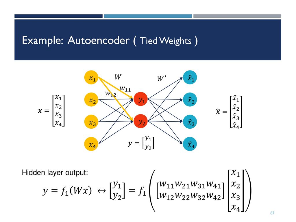
그림 출처: Sildeplayer
Tied AutoEncoder를 살펴보게 되면 Input -> Hidden Space로 가능 Weight와 Hidden Space -> Decoder로 가는 Weight가 비슷한 AutoEncoder를 의미하게 된다.
만약, Input -> Hidden Space로 Mapping하는 Weight를 W라 하고, Hidden Space -> Decoder로 가는 Weight를 \(W^T\)라고 하면, Linear ExtremeLearningMachine Autoencoder와 같다고 할 수 있다.
NonLinear ExtremeLearningMachine는 Weight의 Initialization에 따라서 Performance가 너무 차이나게 되고, Linear ExtremeLearningMachine은 Tied AutoEncoder로서 Modeling하여 사용하는 것이 Performance가 더 좋았다.
Tied AutoEncoder Code
1
2
3
4
5
6
7
8
9
10
11
12
13
14
15
16
17
18
19
20
21
22
23
24
25
26
27
28
29
30
31
32
33
34
import torch, torch.nn as nn, torch.nn.functional as F

# tied auto encoder using functional calls => 3 Layer Tied AutoEncoder
class TiedAutoEncoderFunctional(nn.Module):
    def __init__(self, inp, hidden_units):
        super().__init__()
        # Share Parameter
        self.param1 = nn.Parameter(torch.nn.init.xavier_uniform_(torch.randn(hidden_units[0], inp)),
                                   requires_grad=True)
        self.param2 = nn.Parameter(torch.nn.init.xavier_uniform_(torch.randn(hidden_units[1], hidden_units[0])),
                                   requires_grad=True)
        self.param3 = nn.Parameter(torch.nn.init.xavier_uniform_(torch.randn(hidden_units[2], hidden_units[1]))
                                   , requires_grad=True)

    def forward(self, input):
        # Encoder
        encoded_feats = F.linear(input, self.param1)
        encoded_feats = F.linear(encoded_feats, self.param2)
        encoded_feats = F.linear(encoded_feats, self.param3)

        # Decoder
        decoder_feats = F.linear(encoded_feats, self.param3.t())
        decoder_feats = F.linear(decoder_feats, self.param2.t())
        reconstructed_output = F.linear(decoder_feats, self.param1.t())

        return reconstructed_output

    def call_hidden_layer(self, input, hidden_layer):
        hidden1_output = F.linear(input, self.param1)
        hidden2_output = F.linear(hidden1_output, self.param2)
        hidden3_output = F.linear(hidden2_output, self.param3)
        hidden_output = [hidden1_output, hidden2_output, hidden3_output]

        return hidden_output[hidden_layer]
참조: 원본코드
참조: Extreme Learning Machine for Regression and Multiclass Classification
참조: Representational Learning with Extreme Learning Machine for Big Data
코드에 문제가 있거나 궁금한 점이 있으면 wjddyd66@naver.com으로 Mail을 남겨주세요.
Leave a comment