
Paper07. Matching Network
Matching Networks for One Shot Learning
Matching Networks for One Shot Learning (https://papers.nips.cc/paper/6385-matching-networks-for-one-shot-learning.pdf)
Matching Networks for One Shot Learning Code(https://github.com/RameshArvind/Pytorch-Matching-Networks)
Abstract
Learning from a few examples remains a key challenge in machine learning. Despite recent advances in important domains such as vision and language, the standard supervised deep learning paradigm does not offer a satisfactory solution for learning new concepts rapidly from little data.
In this work, we employ ideas from metric learning based on deep neural features and from recent advances that augment neural networks with external memories. Our framework learns a network that maps a small labelled support set and an unlabelled example to its label, obviating the need for fine-tuning to adapt to new class types.
We then define one-shot learning problems on vision (using Omniglot, ImageNet) and language tasks. Our algorithm improves one-shot accuracy on ImageNet from 87.6% to 93.2% and from 88.0% to 93.8% on Omniglot compared to competing approaches. We also demonstrate the usefulness of the same model on language modeling by introducing a one-shot task on the Penn Treebank.
다른 Few-shot learning의 Paper와 동일한 문제를 지적하고 있다. 적은 Sample로서 Model을 Training하는 것은 아직 잘 수행되지 않고 있다는 것 이다. Matching Networks는 Siamese Network와 마찬가지로, 적은 Sample로서 Model을 Tarining하기 위한 방법 중 하나이며, 중요한 것은 External Memories를 사용한 다는 것과 Metric Learning이라는 것 이다.
즉, 현재 PreTrain된 Model이 없는 상황에서 잘 수행 될 수 있는 Network라고 생각이 든다.
Model
Matching을 살펴보면 다음과 같은 형태를 띄고 있다.
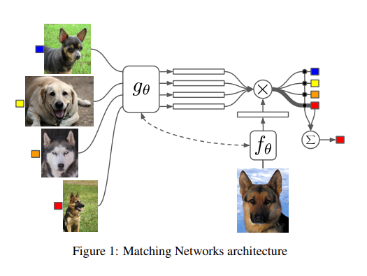
Model의 Architecture를 간단하게 살펴보면 Support set을 Embedding하는 Function \(g_{\theta}\)가 존재하게 되고, Target set을 Embedding하는 Function \(f_{\theta}\)가 존재하게 된다.
위의 두 Embedding된 Feature로부터 Metric기반으로 어느 Support Set에 가까운지 측정하게 되고 이러한 Metric은 Cosine similarity를 선택하게 되었다. => Cosine Similarity이므로 어느 Support에 가까운지 Attention 기법과 같이 작동한다고 얘기하고 있다.
또 중요한 것은 Abstract에서도 설명하였듯이 External Memories를 사용하게 되는데 이는 단순히 Target image 하나만 사용하는 것이 아니라 Support Set을 활용하여 Embedding을하는데 이때 LSTM기반의 Network를 사용하게 되어서 이다.
논문에서는 간단하게 Support set \(S\)가 주어졌을 때 함수 \(C_S\)(Mapping Function or Classifier)를 정의하도록 \(S \rightarrow C_{S}(\cdot)\)을 구하는 것을 목적으로 하고 있다.
Model Architecture
Model Architecture를 설명하기 전에 많이 사용하는 Notation을 정의하면 다음과 같다.
- \(S = {(x_i, y_i)}_{i=1}^{k}\): Support Set
- \(\hat{x}\): Target input
- \(\hat{y}\): Target output
- \(a(\cdot)\): Attention Mechanism
Model설명에서 \(S \rightarrow C_{S}(\cdot)\)을 목표로 하였다. 이것을 위의 Notation을 활용하여 좀 더 자세히 적으면 \(S \rightarrow C_{S}(\hat{x})\)로서 적을 수 있다. 즉, Support set을 활용하여 Target input에 대한 Mapping or Classification을 수행하는 것 이다.
이러한 식을 논문에서는 \(P(\hat{y}|\hat{x},S)\)로서 다시 정의하였다. 즉, Support set과 Target Input이 Input으로 들어오는 경우 Target Label 을 출력하는 확률을 Maximize하도록 Training하게 될 것이며, P는 논문에서 사용하는 Matching Network가 될 것 이다.
위와 같이 Notation이 정의되어 있을 때 논문에서 사용한 Model은 다음과 같이 정의된다.
$$\hat{y} = \sum_{i=1}^k a(\hat{x}, x_i)y_i$$
위의 식에서 중요하게 살펴볼 것은 \(a(\cdot)\)이다. 위의 Notation에서 정의하였듯이 Attention Mechanism으로서 논문에서는 KDE(Kernel Density Estimation)처럼 작동하여 non-parametric이므로 \(C_{S}(\hat{x})\)가 더 유연하고 어떤 support set에서도 잘 적용될 수 있다고 설명하고 있다.
또한, Target input이 Support set중 similarity가 가까운 순으로서 Distance를 정렬할 수 있으므로 K neaarest neighbors처럼 작동한다고 설명할수도 있다. (왜 similarity라하는 지는 The Attention Kernel에서 설명)
The Attention Kernel
$$ a(\hat{x}, x_i) = e^{c(f(\hat{x}), g(x_i))} / \sum_{j=1}^k e^{c(f(\hat{x}), g(x_j))} $$
- \(g(\cdot)\): Support Embedding Function
- \(f(\cdot)\): Target Embedding Function
- \(c(\cdot)\): Cosine Distance
위의 식을 살펴보게 되면, Embedding된 Space상에서 Cosine Distance를 구하고 이에 대하여 Softmax로서 결과를 출력하고 있다. 즉, Target input은 모든 Support input과의 Simialirty를 구하게 되고 각각에 대하여 어느정도 닮았는지 Softmax로서 나타내게 된다. 따라서, Attention과 같은 효과를 내게 된다.
논문에서 위와 같은 분류함수(\(\hat{y} = \sum_{i=1}^k a(\hat{x}, x_i)y_i\))는 Discrimiative하다고 설명하고 있다. 개인적인 해석은 만약 \(y_i\)가 Multi Label이라고 생각하면, 해당 Label을 제외하고 다른 모든 Label과의 Distance는 멀어지게 Training이 될 것 이다. 이런 경우 해당 Label과 다른 Label끼리는 Distance는 가까워질 수 있다는 것 이다. 이렇기 때문에 분류함수가 Discriminative하다고 생각한다.
\(S\)와 \(\hat{x}\)가 주여졌을 경우, \(C_{S}(\hat{x})\)는 \(\hat{y}=y\)인 경우에는 충분히 정렬되고(aligned), 나머지에 대해서는 비정렬(misaligned) 된다는 것 이다. 이러한 Loss는 Neighborhood Component Analysis (NCA), triplet loss, large margin nearest neighbor와 관련된다.
하지만, 논문에서는 해당되는 Label에 대해서만 잘 Classify하는 것도 충분히 성능이 좋다고 이야기 하고 있고, 또한 loss가 쉽고, 미분이 가능하므로 end-to-end로서 잘 학습할 수 있다고 설명하고 있다. 또한, misaligned되는 것에 대해서도 precisely aligned되게 optimize가 가능하면 성능 향상에 많은 도움이 될 것이라고 한계점으로서 이야기하고 있다.
참조
- \(g(\cdot)\)과 \(f(\cdot)\)은 다른 Model을 사용하여도 되고, 같은 Model을 사용하여도 된다고 얘기하고 있다.
- 개인적인 생각으로는 Layer를 더 쌓거나 Feature Space상에서 Decision Boundary를 적용하는 것이 아닌 KDE를 통하여 어떤 Support set과 비슷한지 similarity를 구하고 그에 해당하는 Label에 Mapping하는 방식(non-parametric)이므로 적은 Dataset인 Few shot Learning에 잘 적용되는 Metric이라고 생각한다.
- Kernel에 대한 설명: Kernel(SVM)
Full Context Embedding
개인적으로 해당 논문을 보면서 가장 중요한 부분 중 하나라고 생각한다.
Object Function은 위에서 \(\text{argmax}_{y} P(y|\hat{x},S)\) 로서 나타내었다. 식을 살펴보게 되면 Support Set S에 의해 Fully Condition한 상태인 것을 알 수 있다.
하지만 The Attention Kernel의 식을 살펴보게 되면, Feature Embedding으로서 Mapping하는 Function은 \(f(\hat{x}), g(x_j)\)로서 Support set과 비종속적으로 Embedding하는 것을 살펴볼 수 있다.
해당 논문에서는 이러한 한계점을 극복하기 위하여 Support set을 활용하여 \(f(\hat{x}), g(x_j) \rightarrow f(\hat{x},S), g(x_j,S)\)로서 표현하여 Embedding을 실시하였다.
The Fully Conditional Embedding g
$$g(x_i, S) = \overrightarrow{h_i}+\overleftarrow{h_i}+g^{'}(x_i) \text{ (}g^{'}\text{: Target Embedding Function)}$$
$$\overrightarrow{h_i}, \overrightarrow{c_i} = LSTM(g^{'}(x_i), \overrightarrow{h_{i-1}}, \overrightarrow{c_{i-1}})$$
$$\overleftarrow{h_i}, \overleftarrow{c_i} = LSTM(g^{'}(x_i), \overleftarrow{h_{i-1}}, \overleftarrow{c_{i-1}})$$
- Support set으로서 \(x_i\)가 들어오게 되면, Embedding Function인 \(g^{'}(x)\)로서 Embedding
- Embedding된 \(g^{'}(x)\)를 이전 모든 Support set을 고려하는 Bidirection LSTM에 적용
- LSTM의 Hidden Size가 \(g^{'}(x)\)의 Size와 동일하다면 \(g(x_i, S) = \overrightarrow{h_i}+\overleftarrow{h_i}+g^{'}(x_i)\)으로서 표현 가능.
즉, 개별적이고 독립적인 \(g^{'}(x)\)가 아니라, 이전 Support set을 고려하게 된다.
The Fully Conditional Embedding f
$$ f(\hat{x}, S) = \text{attLSTM}(f'(\hat{x}), g(S), K) \text{ (K: steps of reads, }f^{'}\text{: Target Embedding Function)}$$
$$\hat{h_k}, c_k = \text{LSTM}(f^{'}(\hat{x}), [h_{k-1}, r_{k-1}], c_{k-1})$$
$$h_k = \hat{h_{k}}+f^{'}(\hat{x})$$
$$r_{k-1} = \sum_{i=1}^{|S|} a(h_{k-1}, g(x_i))g(x_i)$$
$$a(h_{k-1}, g(x_i)) = \text{softmax}(h^T_{k-1} g(x_i))$$
- \(g(S)\): Embedding function g applied to each element \(x_i\) from the set S.
위의 식을 살펴보게 되면, 결과적으로 단순히 Hidden Space Mapping이 아닌, LSTM + Attention을 사용하여 Target Input을 Support Input을 고려하여 값을 변형하게 된다.
Training Strategy
$$\theta = \arg \max_\theta E_{L \sim T} \big[ E_{S \sim L, B \sim L} \big[ \sum_{(x, y) \in B} \log P_\theta (y | x, S) \big] \big]$$
- \(T\): Task
- \(L\): 가능한 Label
- \(B\): Batch
위의 식을 해석하면 다음과 같다.
- \(T\)로부터 \(L\)을 Sampling한다.
- \(L\)로부터 Batch Set과 Support Set을 Sampling한다.
- \(B\)의 Label을 Support set을 활용하여 최소화하도록 Model을 Training한다.
Maching Network Code
1
2
3
4
5
6
7
8
9
10
11
12
13
import torch
import torch.nn as nn
import torch.nn.functional as F

import numpy as np
import pandas as pd
import os
from sklearn.preprocessing import MinMaxScaler
from sklearn.model_selection import train_test_split
from tqdm.notebook import tqdm

torch.manual_seed(42)
device = torch.device("cuda:1" if torch.cuda.is_available() else "cpu")
Dataset
DataLoad
1
2
3
4
5
6
7
8
9
10
11
12
file_path = '../EW/'

# Change Diagnosis
def change_dx(dx):
    ctlDxchange = [1, 4, 6]
    adDxChange = [2, 3, 5]

    if dx in ctlDxchange:
        return 0

    elif dx in adDxChange:
        return 1
1
2
3
4
5
6
7
8
9
10
11
12
13
14
15
16
17
18
19
20
# Merge Label with ROI Dataset
roi = pd.read_csv(os.path.join(file_path,'T1/ROI/merge_roi.csv'), index_col=0)
label = pd.read_csv(os.path.join(file_path,'Label.csv'), encoding='cp949')
label = label[['SUBJNO', 'DXGROUP']]
label = label[label['DXGROUP'].notna()]
label['DXGROUP'] = label['DXGROUP'].apply(lambda x:change_dx(x))
label.columns = ['Subject','Label']

roi = pd.merge(roi,label,on='Subject', how='left')
roi = roi[roi['Label'].notna()]
print('Num of ROI Nan: ', roi.isna().sum().sum())

# Preprocess MinMax Normalization
std_scaler = MinMaxScaler()
std_scaler.fit(roi[roi.columns[1:-1]])
output = std_scaler.transform(roi[roi.columns[1:-1]])

roi[roi.columns[1:-1]] = output

roi.head()
1
Num of ROI Nan:  0
| Subject | rh_bankssts_area | rh_caudalanteriorcingulate_area | rh_caudalmiddlefrontal_area | rh_cuneus_area | rh_entorhinal_area | rh_fusiform_area | rh_inferiorparietal_area | rh_inferiortemporal_area | rh_isthmuscingulate_area | ... | wm-rh-rostralmiddlefrontal | wm-rh-superiorfrontal | wm-rh-superiorparietal | wm-rh-superiortemporal | wm-rh-supramarginal | wm-rh-frontalpole | wm-rh-temporalpole | wm-rh-transversetemporal | wm-rh-insula | Label | |
|---|---|---|---|---|---|---|---|---|---|---|---|---|---|---|---|---|---|---|---|---|---|
| 0 | 18 | 0.2850 | 0.696710 | 0.461082 | 0.741722 | 0.475524 | 0.432978 | 0.358528 | 0.264861 | 0.953125 | ... | 0.458181 | 0.609221 | 0.794185 | 0.928987 | 0.844889 | 0.206708 | 0.125912 | 0.372314 | 0.805201 | 0.0 |
| 1 | 19 | 0.6550 | 0.532189 | 0.381926 | 0.705960 | 0.650350 | 0.935502 | 0.546492 | 0.809775 | 0.560938 | ... | 1.000000 | 0.999563 | 0.800884 | 1.000000 | 0.912310 | 0.260884 | 0.192380 | 0.503821 | 0.507652 | 1.0 |
| 2 | 29 | 0.1775 | 0.413448 | 0.132586 | 0.556291 | 1.000000 | 0.332025 | 0.159441 | 0.174373 | 0.479688 | ... | 0.238088 | 0.418293 | 0.586868 | 0.432937 | 0.556274 | 0.617220 | 0.190219 | 0.516799 | 0.533779 | 1.0 |
| 3 | 32 | 0.5125 | 0.366237 | 0.308707 | 0.406623 | 0.230769 | 0.216489 | 0.191957 | 0.554822 | 0.606250 | ... | 0.054872 | 0.262167 | 0.558797 | 0.312242 | 0.447998 | 0.022573 | 0.223994 | 0.249892 | 0.503987 | 1.0 |
| 4 | 33 | 0.3600 | 0.429185 | 0.032322 | 0.000000 | 0.451049 | 0.378015 | 0.290074 | 0.721268 | 0.195312 | ... | 0.712447 | 0.505076 | 0.582903 | 0.409905 | 0.637618 | 0.000000 | 0.891651 | 0.353136 | 0.468153 | 0.0 |
5 rows × 335 columns
Make 1-shot 2-Way Dataset
하고자 하는 Classification의 Category는 2개 이므로 1-shot 2-way Dataset을 구축하게 된다.
1
2
3
4
5
6
7
8
9
10
11
12
13
14
15
16
17
18
19
20
21
22
23
24
25
26
27
28
29
30
31
32
33
34
35
36
37
38
39
40
# Split NL & AD
nl_roi = roi[roi['Label']==0]
ad_roi = roi[roi['Label']==1]

# Split Train 75%, Test 25%
train_nl, test_nl= train_test_split(nl_roi, random_state=42)
train_ad, test_ad= train_test_split(ad_roi, random_state=42)

# Split Train 80%, Dev 20%
train_nl, dev_nl = train_test_split(train_nl, random_state=42, test_size=0.2)
train_ad, dev_ad = train_test_split(train_ad, random_state=42, test_size=0.2)

# Make One-shot 2-way Dataset Dict
# Train Dict
train_dict = []

for i in tqdm(range(len(train_nl)),desc='Make Train Dict'):
    for j in range(len(train_ad)):
        for k in range(i+1, len(train_nl)):
            for d in range(j+1, len(train_ad)):
                train_dict.append({'nl_index': i, 'ad_index': j, 'target_nl_index': k, 'target_ad_index': d})

# Dev Dict
dev_dict = []

for i in tqdm(range(len(dev_nl)),desc='Make Dev Dict'):
    for j in range(len(dev_ad)):
        for k in range(i+1, len(dev_nl)):
            for d in range(j+1, len(dev_ad)):
                dev_dict.append({'nl_index': i, 'ad_index': j, 'target_nl_index': k, 'target_ad_index': d})


# Teset Dict
test_dict = []

for i in tqdm(range(len(test_nl)), desc='Make Test Dict'):
    for j in range(len(test_ad)):
        for k in range(i+1, len(test_nl)):
            for d in range(j+1, len(test_ad)):
                test_dict.append({'nl_index': i, 'ad_index': j, 'target_nl_index': k, 'target_ad_index': d})
Data Loader
For Batch Dataset
1
2
3
4
5
6
7
8
9
10
11
12
13
14
15
16
17
18
19
20
21
22
23
24
25
26
27
28
29
30
31
32
33
34
35
36
37
38
39
40
41
from torch.utils.data.dataset import Dataset
import random

class OneShotDataset(Dataset):
    def __init__(self, nl_roi, ad_roi, dict_list):
        self.nl_roi = nl_roi
        self.ad_roi = ad_roi
        self.dict_list = dict_list

    def __getitem__(self, index):
        nl_index = self.dict_list[index]['nl_index']
        ad_index = self.dict_list[index]['ad_index']

        # Select Target NL
        r = random.choice([0,1])
        if r == 0:
            target_index = self.dict_list[index]['target_nl_index']
            target_value = self.nl_roi.iloc[target_index,1:-1].values
            target_label = self.nl_roi.iloc[target_index,-1]
        # Select Target AD
        else:
            target_index = self.dict_list[index]['target_ad_index']
            target_value = self.ad_roi.iloc[target_index,1:-1].values
            target_label = self.ad_roi.iloc[target_index,-1]

        # Support Set
        r = random.choice([0,1])
        if r == 0:
            support_value = np.row_stack((nl_roi.iloc[nl_index,1:-1].values, ad_roi.iloc[ad_index,1:-1].values))
            support_labels = np.array([nl_roi.iloc[nl_index,-1], ad_roi.iloc[ad_index,-1]])
        else:
            support_value = np.row_stack((ad_roi.iloc[ad_index,1:-1].values, nl_roi.iloc[nl_index,1:-1].values))
            support_labels = np.array([ad_roi.iloc[ad_index,-1], nl_roi.iloc[nl_index,-1]])

        return (torch.from_numpy(support_value).float(),
            torch.from_numpy(support_labels).long().unsqueeze(-1),
            torch.from_numpy(target_value).float(),
            target_label)

    def __len__(self):
        return len(self.dict_list)
Matching Network Model
Embedding Layer
Input을 Feature Space상에서 Mapping하는 작업이다. Input의 Feature는 333이고, Feature Sapce상에서는 10 Dimension으로서 Mapping되게 ANN으로서 구성하였다.
- Activation Function: ReLU
- Dropout
1
2
3
4
5
6
7
8
9
10
11
12
class Single_Layer(nn.Module):
    def __init__(self, in_hidden, out_hidden, dropout_probality=0.2):
        super().__init__()
        self.linear = nn.Linear(in_hidden, out_hidden)
        self.ReLU = nn.ReLU()
        self.dropout = nn.Dropout(dropout_probality) # Dropout to add regularization and improve model generalization

    def forward(self, X):
        x = self.linear(X)
        x = self.ReLU(x)
        x = self.dropout(x)
        return x
1
2
3
4
5
6
7
8
9
10
11
12
13
14
15
16
17
18
19
20
21
22
23
24
25
26
class Embedding(nn.Module):

    def __init__(self, embedding_size=10, dropout_probality=0.2):
        super().__init__()
        self.layer1 = Single_Layer(333, 200, dropout_probality= dropout_probality)
        self.layer2 = Single_Layer(200, 100, dropout_probality= dropout_probality)
        self.dense = nn.Linear(100, embedding_size)
        self.dropout = nn.Dropout(dropout_probality)
        self.embedding_size = embedding_size

        # Weight Initializer
        self.layer1.apply(self.init_weights)
        self.layer2.apply(self.init_weights)

    # Weight Initializer => Xavier
    def init_weights(self, m):
        if type(m) == nn.Linear:
            torch.nn.init.xavier_uniform_(m.weight)

    def forward(self, x):
        x = self.layer1(x)
        x = self.layer2(x)
        x = self.dense(x)
        x = self.dropout(x)

        return x
The Fully Conditional Embedding - Target Set
$$ f(\hat{x}, S) = \text{attLSTM}(f'(\hat{x}), g(S), K) \text{ (K: steps of reads, }f^{'}\text{: Target Embedding Function)}$$
$$\hat{h_k}, c_k = \text{LSTM}(f^{'}(\hat{x}), [h_{k-1}, r_{k-1}], c_{k-1})$$
$$h_k = \hat{h_{k}}+f^{'}(\hat{x})$$
$$r_{k-1} = \sum_{i=1}^{|S|} a(h_{k-1}, g(x_i))g(x_i)$$
$$a(h_{k-1}, g(x_i)) = \text{softmax}(h^T_{k-1} g(x_i))$$
- \(g(S)\): Embedding function g applied to each element \(x_i\) from the set S.
1
2
3
4
5
6
7
8
9
10
11
12
13
14
15
16
17
18
19
20
21
22
class FullyConditionalEmbeddingTarget(nn.Module):
    def __init__(self, embedding_size, processing_steps=10):
        super().__init__()
        self.lstm_cell = torch.nn.LSTMCell(embedding_size, embedding_size)
        self.processing_steps = processing_steps
        self.embedding_size = embedding_size
        self.attn_softmax = nn.Softmax(dim=1)

    def forward(self, target_encoded, support_encoded):
        batch_size, num_sample, _ = support_encoded.shape
        cell_state_prev = torch.zeros(batch_size, self.embedding_size).to(device)
        hidden_state_prev = torch.sum(support_encoded, dim=1) / num_sample

        for i in range(self.processing_steps):
            hidden_out, cell_out = self.lstm_cell(target_encoded, (hidden_state_prev, cell_state_prev))
            hidden_out = hidden_out + target_encoded
            attn = self.attn_softmax(torch.bmm(support_encoded, hidden_out.unsqueeze(2)))
            attended_values = torch.sum(attn * support_encoded, dim=1)
            hidden_state_prev = hidden_out + attended_values
            cell_state_prev = cell_out

        return hidden_out
The Fully Conditional Embedding - Support Images
$$g(x_i, S) = \overrightarrow{h_i}+\overleftarrow{h_i}+g^{'}(x_i) \text{ (}g^{'}\text{: Target Embedding Function)}$$
$$\overrightarrow{h_i}, \overrightarrow{c_i} = LSTM(g^{'}(x_i), \overrightarrow{h_{i-1}}, \overrightarrow{c_{i-1}})$$
$$\overleftarrow{h_i}, \overleftarrow{c_i} = LSTM(g^{'}(x_i), \overleftarrow{h_{i-1}}, \overleftarrow{c_{i-1}})$$
1
2
3
4
5
6
7
8
9
10
11
12
13
14
15
16
17
18
19
20
21
22
23
24
25
class FullyConditionalEmbeddingSupport(nn.Module):
    def __init__(self, embedding_size):
        super().__init__()
        self.embedding_size = embedding_size
        self.bidirectionalLSTM = nn.LSTM(input_size=embedding_size, hidden_size=embedding_size, bidirectional=True, batch_first=True)

    def initialize_hidden(self, batch_size):
        #Initialize the states needed for our bi-directional LSTM
        hidden_state = torch.zeros(2, batch_size, self.embedding_size).to(device)
        cell_state = torch.zeros(2, batch_size, self.embedding_size).to(device)
        return (hidden_state, cell_state)

    def forward(self, support_embeddings):
        batch_size, num_images, _ = support_embeddings.shape
        # Initialize states
        lstm_states = self.initialize_hidden(batch_size)
        # Get the LSTM Outputs
        support_embeddings_contextual, internal_states = self.bidirectionalLSTM(support_embeddings, lstm_states)
        # Get the forward and backward outputs
        support_embeddings_contextual = support_embeddings_contextual.view(batch_size, num_images, 2, self.embedding_size)
        # Add the forward and backward outputs
        support_embeddings_contextual = torch.sum(support_embeddings_contextual, dim=2)
        # Add the skip connection to our output
        support_embeddings_contextual = support_embeddings_contextual + support_embeddings
        return support_embeddings_contextual
Cosine Distance
$$\text{similarity} = cos(\theta) = \frac{A \cdot B}{\| A \| \| B \|} = \frac{\sum_{i=1}^n A_i B_i}{\sqrt{\sum_{i=1}^n A_i^2}\sqrt{\sum_{i=1}^n B_i^2}}$$
1
2
3
4
5
6
7
8
9
10
11
12
13
14
15
16
17
18
19
20
21
22
class CosineDistance(nn.Module):

  def __init__(self):
        super().__init__()

  def forward(self, target_image, support_images):
    # Embedding Feature 기준으로 Normalization => Support Image의 경우에는 Batch, Num of Class, Embedding
    # support_image.shape => torch.Size([batch_size, 2(Num of Class), 10(Embedding Size)])
    support_images_normed = F.normalize(support_images, p=2, dim=2)
    # the 'p=2' param represents squared norm
    # support_image.shape => torch.Size([batch_size, 10])
    target_image_normed = F.normalize(target_image, p=2, dim=1)
    # This will cause the dimensions to be [batch_size, 10, 1]
    target_image_normed = target_image_normed.unsqueeze(dim=1).permute(0, 2, 1)

    similarities = torch.bmm(support_images_normed, target_image.unsqueeze(1).permute(0, 2, 1))
    # torch.bmm = batch matrix multiply
    # [batch_size, 2(Num of Class), 10(Embedding Size)] @ [batch_size, 10(Embedding Size), 1]
    # the output shape is [batch_size, 2(Num of Class), 1]
    similarities = similarities.squeeze(dim=2)
    # remove last dimension
    return similarities
Label Category => One-Hot-Encoding
1
2
3
4
5
6
7
8
9
# Taken from @activatedgeeks's answer from https://stackoverflow.com/questions/44461772/creating-one-hot-vector-from-indices-given-as-a-tensor
class ConvertOneHot(nn.Module):
    def __init__(self):
        super().__init__()

    def forward(self, labels, num_classes):
        batch_size, num_images, _ = labels.size()
        one_hot_labels = torch.Tensor(batch_size, num_images, num_classes).to(labels.device).float().zero_()
        return one_hot_labels.scatter(2, labels, 1)
Matching Network
- Paper와 같이 The Fully Conditional Embedding을 사용하게 된다면 다음과 같은 과정을 거치게 된다.
- 1) Input -> Embedding Layer -> Feature Embedding
- 2) Support Set => Support Feature Embedding(Input) -> Bidirection LSTM(FullyConditionalEmbeddingSupport) -> Support Feature Embedding(Output)
- 3) Target Set => Target Feature Embedding, Support Feature Embedding(Output)-> Attention LSTM(FullyConditionalEmbeddingTarget) -> Target Feature Embedding(Output)
- Support Set을 활용하여 Feature Embedding된 Support Feature Embedding과 Target Feature Embedding의 Cosine Similarity를 구한다. (distances)
- Softmax Function을 사용하여 distance에 대한 Attention을 구한다.
- Support Labels와 Attention의 결과를 활용하여 Prediction의 결과를 구한다.
1
2
3
4
5
6
7
8
9
10
11
12
13
14
15
16
17
18
19
20
21
22
23
24
25
26
27
28
29
30
31
32
33
34
35
36
37
38
39
40
class MatchingNet(nn.Module):

  def __init__(self, embedding_size=10, dropout_probality=0.2, use_fce=True):
    super().__init__()
    self.attn = nn.Softmax(dim=1)
    self.embedding = Embedding(embedding_size=embedding_size, dropout_probality=dropout_probality)
    self.distance = CosineDistance()
    self.use_fce = use_fce
    self.onehotconverter = ConvertOneHot()
    if self.use_fce:
      self.full_conditional_embedding_support = FullyConditionalEmbeddingSupport(embedding_size=embedding_size)
      self.full_conditional_embedding_target = FullyConditionalEmbeddingTarget(embedding_size=embedding_size)

  def forward(self, support_images, support_labels, target_image):
    batch_size, num_images, _ = support_labels.size()

    # Get the image encodings from convolutional embedding
    target_image_encoded = self.embedding(target_image)
    support_images_encoded = self.embedding(support_images)

    if self.use_fce:
      # Get the support images embedding with context
      support_images_encoded = self.full_conditional_embedding_support(support_images_encoded)

      # Get the target image embedding with context
      target_image_encoded = self.full_conditional_embedding_target(target_image_encoded, support_images_encoded)

    # Get the cosine distances between target image and the support images
    distances = self.distance(target_image_encoded, support_images_encoded)
    # Get the attention value based on the distances
    attention = self.attn(distances)
    # Convert the labels into one hot vectors
    support_set_one_hot_labels = self.onehotconverter(support_labels, num_images)

    # Get the prediction logits by attention * one-hot-labels (automatically summed due to the unsqueeze operation)
    prediction_logits = torch.bmm(attention.unsqueeze(1), support_set_one_hot_labels).squeeze()

    # Get the final labels for predictions
    _, prediction_labels = torch.max(prediction_logits, 1)
    return prediction_logits, prediction_labels
Check Matching Network Architecture
1
2
3
4
5
6
7
8
9
10
11
12
13
14
15
16
17
18
19
20
21
22
23
matching_net_trial = MatchingNet(333, dropout_probality=0.1, use_fce=True)
print("Model Summary")
print(matching_net_trial)
epochs = 10

support_images = torch.rand(32, 2, 333)
target_image = torch.rand(32, 333)
support_labels = torch.LongTensor(32, 2, 1) % 20
target_labels = torch.LongTensor(32) % 20

matching_net_trial.to(device)
support_images = support_images.to(device)
support_labels = support_labels.to(device)
target_image = target_image.to(device)
target_labels = target_labels.to(device)
optimizer = torch.optim.Adam(matching_net_trial.parameters(), lr=0.001)
for epoch in range(epochs):
  logits, predictions = matching_net_trial(support_images, support_labels,target_image)
  loss = F.cross_entropy(logits, target_labels)
  print(loss.item())
  optimizer.zero_grad()
  loss.backward()
  optimizer.step()
1
2
3
4
5
6
7
8
9
10
11
12
13
14
15
16
17
18
19
20
21
22
23
24
25
26
27
28
29
30
31
32
33
34
35
36
37
Model Summary
MatchingNet(
  (attn): Softmax(dim=1)
  (embedding): Embedding(
    (layer1): Single_Layer(
      (linear): Linear(in_features=333, out_features=200, bias=True)
      (ReLU): ReLU()
      (dropout): Dropout(p=0.1, inplace=False)
    )
    (layer2): Single_Layer(
      (linear): Linear(in_features=200, out_features=100, bias=True)
      (ReLU): ReLU()
      (dropout): Dropout(p=0.1, inplace=False)
    )
    (dense): Linear(in_features=100, out_features=333, bias=True)
    (dropout): Dropout(p=0.1, inplace=False)
  )
  (distance): CosineDistance()
  (onehotconverter): ConvertOneHot()
  (full_conditional_embedding_support): FullyConditionalEmbeddingSupportImages(
    (bidirectionalLSTM): LSTM(333, 333, batch_first=True, bidirectional=True)
  )
  (full_conditional_embedding_target): FullyConditionalEmbeddingTargetImage(
    (lstm_cell): LSTMCell(333, 333)
    (attn_softmax): Softmax(dim=1)
  )
)
0.4925367534160614
0.4794721305370331
0.4599059224128723
0.4850090742111206
0.5028786063194275
0.43996888399124146
0.43130460381507874
0.43095457553863525
0.4187224805355072
0.42587724328041077
Training & Test Model
Evaluate Model
For Devset & Testset
1
2
3
4
5
6
7
8
9
10
11
12
13
14
15
16
17
18
19
20
21
22
23
24
25
26
27
28
29
30
31
32
33
34
35
def evaluate_model(model, nl, ad, dict_list, batch_size=20):
    model.eval() # Set the model in eval mode so as ensure Dropout and BatchNorm layers operate in Evaluation mode
    # Set up our dataloaders
    dataset = OneShotDataset(nl, ad, dict_list)
    dataset_loader = torch.utils.data.DataLoader(dataset=dataset,
                                                  batch_size=batch_size,
                                                  num_workers=4,
                                                  shuffle=False)

    # Run in no_grad mode to speed up inference
    with torch.no_grad():
        # Placeholders to accumulate the metrics across batches
        total_accuracy = 0
        total_loss = 0

        for iteration, (support_images, support_labels, images, labels) in enumerate(dataset_loader):
            # Move Data to GPU
            support_batch_torch = support_images.to(device)
            support_labels_torch = support_labels.to(device)
            target_images_torch = images.to(device)
            target_labels_torch =labels.to(device).long()

            # Perform inference via our model
            logits, predictions = model(support_batch_torch, support_labels_torch, target_images_torch)
            # Calculate loss and accuracy
            loss = F.cross_entropy(logits, target_labels_torch)
            accuracy = torch.mean((predictions == target_labels_torch).float())

            # Accumulate the metrics
            total_loss = total_loss + loss.item()
            total_accuracy = total_accuracy + accuracy.item()

        accuracy = total_accuracy/(iteration+1)
        loss = total_loss/(iteration+1)
        return accuracy, loss
Hyperparameter & Model Check
1
2
3
4
5
6
7
epochs = 60 #@param {type: "slider", min: 1, max: 100}
batch_size = 20 #@param {type: "slider", min: 20, max: 200}
iterations = 10000 #@param {type: "slider", min: 500, max: 10000}
lr = 0.0001 #@param ["0.1", "0.01", "0.001", "0.0001"] {type:"raw", allow-input: true}
embedding_size = 10 #@param {type: "slider", min: 64, max: 512}
dropout_probality=0.1 #@param {type: "slider", min: 0, max: 1, step: 0.1}
use_fce = True #@param ["True", "False"] {type:"raw"}
1
2
3
4
# Define the model
matching_net = MatchingNet(embedding_size=embedding_size, dropout_probality=dropout_probality, use_fce=use_fce)
print("Model Summary")
print(matching_net)
1
2
3
4
5
6
7
8
9
10
11
12
13
14
15
16
17
18
19
20
21
22
23
24
25
26
27
Model Summary
MatchingNet(
  (attn): Softmax(dim=1)
  (embedding): Embedding(
    (layer1): Single_Layer(
      (linear): Linear(in_features=333, out_features=200, bias=True)
      (ReLU): ReLU()
      (dropout): Dropout(p=0.1, inplace=False)
    )
    (layer2): Single_Layer(
      (linear): Linear(in_features=200, out_features=100, bias=True)
      (ReLU): ReLU()
      (dropout): Dropout(p=0.1, inplace=False)
    )
    (dense): Linear(in_features=100, out_features=10, bias=True)
    (dropout): Dropout(p=0.1, inplace=False)
  )
  (distance): CosineDistance()
  (onehotconverter): ConvertOneHot()
  (full_conditional_embedding_support): FullyConditionalEmbeddingSupportImages(
    (bidirectionalLSTM): LSTM(10, 10, batch_first=True, bidirectional=True)
  )
  (full_conditional_embedding_target): FullyConditionalEmbeddingTargetImage(
    (lstm_cell): LSTMCell(10, 10)
    (attn_softmax): Softmax(dim=1)
  )
)
Model Train
1
2
3
4
5
6
7
8
9
10
11
12
13
14
15
16
17
18
19
20
21
22
23
24
25
26
27
28
29
30
31
32
33
34
35
36
37
38
39
40
41
42
43
44
45
46
47
48
49
50
51
52
53
54
55
56
57
58
59
60
# Move the model to GPU
matching_net.to(device)
# Create the optimizer
optimizer = torch.optim.Adam(matching_net.parameters(), lr=lr)
# placeholders to store our best performing metrics on Dev Set
best_dev_loss = 0
best_dev_accuracy = 0

print("Beginning Training..")

for epoch in range(epochs):
    matching_net.train() # Set our model in train mode

    # Placeholder variables to help track epoch loss and accuracy
    total_loss = 0
    total_accuracy = 0

    # Define our dataset and dataloader
    train_dataset = OneShotDataset(train_nl, train_ad, train_dict)
    train_dataset_loader = torch.utils.data.DataLoader(dataset=train_dataset,
                                                  batch_size=batch_size,
                                                  num_workers=4,
                                                  shuffle=False)
    # Main training loop
    for iteration, (support_images, support_labels, images, labels) in enumerate(train_dataset_loader):
        # Move our data to GPU
        support_batch_torch = support_images.to(device)
        support_labels_torch = support_labels.to(device)
        target_images_torch = images.to(device)
        target_labels_torch =labels.to(device).long()
        # Get the predictions and logits from our model
        logits, predictions = matching_net(support_batch_torch, support_labels_torch, target_images_torch)

        # Calculate loss and accuracy in current iteration
        loss = F.cross_entropy(logits, target_labels_torch)
        accuracy = torch.mean((predictions == target_labels_torch).float())

        # Accumulate the values
        total_loss = total_loss + loss.item()
        total_accuracy = total_accuracy + accuracy.item()

        # Perform Backpropagation
        optimizer.zero_grad()
        loss.backward()
        optimizer.step()

    total_accuracy = total_accuracy/(iteration+1)
    total_loss = total_loss/(iteration+1)

    # Run the model on Dev Set to evaluate performance on unseen data (every 3 epochs)
    if epoch%3 == 0:
        dev_accuracy, dev_loss = evaluate_model(matching_net, dev_nl, dev_ad, dev_dict)
        print(f"--In epoch - {epoch} Dev Set Accuracy - {dev_accuracy} Loss - {dev_loss}")

        # Save the best performing model across all the epochs
        if not best_dev_loss or dev_loss < best_dev_loss:
            print(f"---Found Better Model to save with Accuracy - {dev_accuracy} and loss - {dev_loss}")
            best_dev_loss = dev_loss
            best_dev_accuracy = dev_accuracy
            torch.save(matching_net.state_dict(), "matching_net-%0.2f-accuracy.pt"%(best_dev_accuracy))
1
2
3
4
5
6
7
8
9
10
11
12
13
14
15
16
17
18
19
20
21
22
23
24
Beginning Training..
--In epoch - 0 Dev Set Accuracy - 0.8333333134651184 Loss - 0.5581295490264893
---Found Better Model to save with Accuracy - 0.8333333134651184 and loss - 0.5581295490264893
--In epoch - 3 Dev Set Accuracy - 1.0 Loss - 0.32173553109169006
---Found Better Model to save with Accuracy - 1.0 and loss - 0.32173553109169006
--In epoch - 6 Dev Set Accuracy - 1.0 Loss - 0.33157289028167725
--In epoch - 9 Dev Set Accuracy - 1.0 Loss - 0.31589415669441223
---Found Better Model to save with Accuracy - 1.0 and loss - 0.31589415669441223
--In epoch - 12 Dev Set Accuracy - 1.0 Loss - 0.3188683092594147
--In epoch - 15 Dev Set Accuracy - 0.8333333134651184 Loss - 0.47293928265571594
--In epoch - 18 Dev Set Accuracy - 0.8888888955116272 Loss - 0.42926275730133057
--In epoch - 21 Dev Set Accuracy - 0.7222222089767456 Loss - 0.5962282419204712
--In epoch - 24 Dev Set Accuracy - 0.7777777910232544 Loss - 0.5358051657676697
--In epoch - 27 Dev Set Accuracy - 0.7777777910232544 Loss - 0.5335798263549805
--In epoch - 30 Dev Set Accuracy - 0.8333333134651184 Loss - 0.4804406762123108
--In epoch - 33 Dev Set Accuracy - 0.8333333134651184 Loss - 0.4794936776161194
--In epoch - 36 Dev Set Accuracy - 0.8333333134651184 Loss - 0.4803601801395416
--In epoch - 39 Dev Set Accuracy - 0.7777777910232544 Loss - 0.5354985594749451
--In epoch - 42 Dev Set Accuracy - 0.944444477558136 Loss - 0.3712233006954193
--In epoch - 45 Dev Set Accuracy - 0.7777777910232544 Loss - 0.5351426601409912
--In epoch - 48 Dev Set Accuracy - 0.7777777910232544 Loss - 0.5349035263061523
--In epoch - 51 Dev Set Accuracy - 0.944444477558136 Loss - 0.3691905736923218
--In epoch - 54 Dev Set Accuracy - 0.8888888955116272 Loss - 0.4241746664047241
--In epoch - 57 Dev Set Accuracy - 0.944444477558136 Loss - 0.36891207098960876
Model Test
1
2
3
4
5
6
matching_net_test = MatchingNet(embedding_size=embedding_size, dropout_probality=dropout_probality, use_fce=use_fce)
matching_net_test.load_state_dict(torch.load("matching_net-%0.2f-accuracy.pt"%(best_dev_accuracy)))
matching_net_test.to(device)
matching_net_test.eval()
test_accuracy, test_loss = evaluate_model(matching_net_test, test_nl, test_ad, test_dict)
print(f"Test Set Accuracy - {test_accuracy} Loss - {test_loss}")
1
Test Set Accuracy - 0.7045454735105688 Loss - 0.6039107089692896
No Use FCE
1
2
3
4
5
6
7
8
9
10
11
12
13
14
15
16
17
18
19
20
21
22
23
24
25
26
27
28
29
30
31
32
33
34
35
36
37
38
39
40
41
42
43
44
45
46
47
48
49
50
51
52
53
54
55
56
57
58
59
60
61
62
63
# Define the model
matching_net = MatchingNet(embedding_size=embedding_size, dropout_probality=dropout_probality, use_fce=False)

# Move the model to GPU
matching_net.to(device)
# Create the optimizer
optimizer = torch.optim.Adam(matching_net.parameters(), lr=lr)
# placeholders to store our best performing metrics on Dev Set
best_dev_loss = 0
best_dev_accuracy = 0

print("Beginning Training..")

for epoch in range(epochs):
    matching_net.train() # Set our model in train mode

    # Placeholder variables to help track epoch loss and accuracy
    total_loss = 0
    total_accuracy = 0

    # Define our dataset and dataloader
    train_dataset = OneShotDataset(train_nl, train_ad, train_dict)
    train_dataset_loader = torch.utils.data.DataLoader(dataset=train_dataset,
                                                  batch_size=batch_size,
                                                  num_workers=4,
                                                  shuffle=False)
    # Main training loop
    for iteration, (support_images, support_labels, images, labels) in enumerate(train_dataset_loader):
        # Move our data to GPU
        support_batch_torch = support_images.to(device)
        support_labels_torch = support_labels.to(device)
        target_images_torch = images.to(device)
        target_labels_torch =labels.to(device).long()
        # Get the predictions and logits from our model
        logits, predictions = matching_net(support_batch_torch, support_labels_torch, target_images_torch)

        # Calculate loss and accuracy in current iteration
        loss = F.cross_entropy(logits, target_labels_torch)
        accuracy = torch.mean((predictions == target_labels_torch).float())

        # Accumulate the values
        total_loss = total_loss + loss.item()
        total_accuracy = total_accuracy + accuracy.item()

        # Perform Backpropagation
        optimizer.zero_grad()
        loss.backward()
        optimizer.step()

    total_accuracy = total_accuracy/(iteration+1)
    total_loss = total_loss/(iteration+1)

    # Run the model on Dev Set to evaluate performance on unseen data (every 3 epochs)
    if epoch%3 == 0:
        dev_accuracy, dev_loss = evaluate_model(matching_net, dev_nl, dev_ad, dev_dict)
        print(f"--In epoch - {epoch} Dev Set Accuracy - {dev_accuracy} Loss - {dev_loss}")

        # Save the best performing model across all the epochs
        if not best_dev_loss or dev_loss < best_dev_loss:
            print(f"---Found Better Model to save with Accuracy - {dev_accuracy} and loss - {dev_loss}")
            best_dev_loss = dev_loss
            best_dev_accuracy = dev_accuracy
            torch.save(matching_net.state_dict(), "No_FCE_matching_net-%0.2f-accuracy.pt"%(best_dev_accuracy))
1
2
3
4
5
6
7
8
Beginning Training..
--In epoch - 0 Dev Set Accuracy - 0.8888888955116272 Loss - 0.6647112369537354
---Found Better Model to save with Accuracy - 0.8888888955116272 and loss - 0.6647112369537354
--In epoch - 3 Dev Set Accuracy - 1.0 Loss - 0.37151992321014404
---Found Better Model to save with Accuracy - 1.0 and loss - 0.37151992321014404
--In epoch - 6 Dev Set Accuracy - 1.0 Loss - 0.34736594557762146
---Found Better Model to save with Accuracy - 1.0 and loss - 0.34736594557762146
--In epoch - 9 Dev Set Accuracy - 0.8888888955116272 Loss - 0.42781704664230347
Test
1
2
3
4
5
6
matching_net_test = MatchingNet(embedding_size=embedding_size, dropout_probality=dropout_probality, use_fce=False)
matching_net_test.load_state_dict(torch.load("No_FCE_matching_net-%0.2f-accuracy.pt"%(best_dev_accuracy)))
matching_net_test.to(device)
matching_net_test.eval()
test_accuracy, test_loss = evaluate_model(matching_net_test, test_nl, test_ad, test_dict)
print(f"Test Set Accuracy - {test_accuracy} Loss - {test_loss}")
1
Test Set Accuracy - 0.8136363788084551 Loss - 0.46823787689208984
FCE를 사용하지 않았을 경우 더 성능이 좋은 것을 알 수 있다. N-way에서 Experiment나 Code는 20way를 적용하였지만, 현재 Task는 Binary Classification이므로 추가적인 Support Set을 활용한 Attention을 적용하는 것은 성능이 더 안 좋은 것을 알 수 있다.
성능은 좋게 나오게 되었지만, 중요한 것은 Matching Network는 Set-to-Set을 해결하기 위한 Model이므로 다른 Model과의 비교 및 각각의 새로운 Dataset에 대하여 어느정도 결과를 보장할 지는 알 수 있는 방법이 없다.
참조: Paper.Matching Networks for One Shot Learning
참조: Code.Matching Networks for One Shot Learning
코드에 문제가 있거나 궁금한 점이 있으면 wjddyd66@naver.com으로 Mail을 남겨주세요.
Leave a comment