
Pytorch-학습 관련 기술들
학습 관련 기술들
Model 구성 시 성능향상을 위해 고려해야 하는 사항에 대해서 알아보자.
아래 링크는 현재 Post에서 구현할 개념을 다룬 내용이다.
NeuralNetwork (5) 학습 관련 기술들
정형화
매우 큰 가중치가 존재한다고 생각하면 그 하나의 가중치에 의해서 Model이 결정되므로 Overfitting된다고 생각할 수 있기 때문이다.
이러한 가중치 감소는 크게 2가지로 나뉘어 질 수 있다.
1) L2 Regularization: 가장 일반적인 regulization 기법입니다. 기존 손실함수(Lold)에 모든 학습파라메터의 제곱을 더한 식을 새로운 손실함수로 씁니다. 아래 식과 같습니다. 여기에서 1/2이 붙은 것은 미분 편의성을 고려한 것이고, λ는 패널티의 세기를 결정하는 사용자 지정 하이퍼파라메터입니다. 이 기법은 큰 값이 많이 존재하는 가중치에 제약을 주고, 가중치 값을 가능한 널리 퍼지도록 하는 효과를 냅니다.
$$W = [w_1, w_2, ... , w_n]$$
$$L_{new} = L_{old} + \frac{\lambda}{2}(w_1^2 + w_2^2 + ... + w_n^2)$$
2) L1 Regularization: 기존 손실함수에 학습파라메터의 절대값을 더해 적용합니다. 이 기법은 학습파라메터를 sparse하게(거의 0에 가깝게) 만드는 특성이 있습니다.
$$L_{new} = L_{old} + \lambda (\left| w_1 \right| + \left| w_2 \right| + ... + \left| w_n \right|)$$
각각의 방식을 그래프로 표현하게 되면 다음과 같다.

즉, L1 Regularization에서 Sparse하다는 것은 Weight가 0으로 될 확률이 높다는 것이다.
Sparse: 전체 w중 0이 많은 경우
위의 공통된 식을 살펴보게 되면 가중치가 큰 곳에 더 큰 Loss를 더해주는 것이 핵심이다.
Loss 가 커지게 되면 Gradinet Descent 를 생각하였을 때 더욱 더 빨리 최소값에 수렴하게 되고 빨리 수렴하게 되면 무한정으로 커지는 것을 막을 수 있다.
Pytorch에서의 Weight Regularization은 weight_decay(\(\lambda\) ) Parameter로 조절할 수 있습니다.
- weight_decay (float, optional) – weight decay (L2 penalty) (default: 0)
Weight_decay는 L2 Regularization으로 적용되므로 L1 Regularization으로 적용시키기 위해서는 명시적으로 손실함수에 식을 추가해야 한다.
Weight Regularization Model
1) CNN Model
1
2
3
4
5
6
7
8
9
10
11
12
13
14
15
16
17
18
19
20
21
22
23
24
class CNN(nn.Module):
    def __init__(self):
        super(CNN,self).__init__()
        self.layer = nn.Sequential(
            nn.Conv2d(1,16,3,padding=1),  # 28 x 28
            nn.ReLU(),
            nn.Conv2d(16,32,3,padding=1), # 28 x 28
            nn.ReLU(),
            nn.MaxPool2d(2,2),            # 14 x 14
            nn.Conv2d(32,64,3,padding=1), # 14 x 14
            nn.ReLU(),
            nn.MaxPool2d(2,2)             #  7 x 7
        )
        self.fc_layer = nn.Sequential(
            nn.Linear(64*7*7,100),
            nn.ReLU(),
            nn.Linear(100,10)
        )

    def forward(self,x):
        out = self.layer(x)
        out = out.view(batch_size,-1)
        out = self.fc_layer(out)
        return out
optimizer = torch.optim.SGD(model.parameters(), lr=learning_rate, weight_decay=0.1)
위의 Code에서 weight_decay=0.1로 설정한다는 것은
L2 Regularization 식에서
$$L_{new} = L_{old} + \frac{\lambda}{2}(w_1^2 + w_2^2 + ... + w_n^2)$$
\(\lambda\) = 0.1로 설정한다는 것 이다.
2) Loss func & Optimizer
1
2
3
4
5
6
7
8
device = torch.device("cuda:0" if torch.cuda.is_available() else "cpu")
print(device)

model = CNN().to(device)
loss_func = nn.CrossEntropyLoss()

# 정형화는 weight_decay로 줄 수 있습니다.
optimizer = torch.optim.SGD(model.parameters(), lr=learning_rate, weight_decay=0.1)
3) Train
1
2
3
4
5
6
7
8
9
10
11
12
13
for i in range(num_epoch):
    for j,[image,label] in enumerate(train_loader):
        x = image.to(device)
        y_= label.to(device)

        optimizer.zero_grad()
        output = model.forward(x)
        loss = loss_func(output,y_)
        loss.backward()
        optimizer.step()

    if i % 10 == 0:
        print(loss)
4) Test
1
2
3
4
5
6
7
8
9
10
11
12
13
14
15
correct = 0
total = 0

with torch.no_grad():
  for image,label in test_loader:
      x = image.to(device)
      y_= label.to(device)

      output = model.forward(x)
      _,output_index = torch.max(output,1)

      total += label.size(0)
      correct += (output_index == y_).sum().float()

  print("Accuracy of Test Data: {}".format(100*correct/total))
Accuracy of Test Data: 12.600160598754883
Dropout
Dropout은 Overfitting을 막기위한 방법으로 뉴럴 네트워크가 학습중일때, 랜덤하게 뉴런을 꺼서 학습함으로써, 학습이 학습용 데이터로 치우치는 현상을 막아준다.

Pytorch에서는 model.train()으로서 Model이 Train상태일 때는 Dropout을 적용하고 model.eval()에서는 Model의 결과를 확인하므로 Dropout을 적용 안한다.
또한 중요한점은 정형화나 Dropout의 기법은 항상 결과가 좋아지지 않는다.
기존의 Model에서 제약을 거는 것 이기 때문에 오버피팅하지 않는 상태에서 정형화나 드롭아웃을 넣으면 오히려 학습이 잘 안되는 결과가 나온다.
Dropout Model
1) CNN Model
torch.nn.Dropout2d(p=0.5, inplace=False)
- p: Dropout 시킬 확률
- inplace: 다른 객체를 반환하지 않고 기존 객체를 수정(Default: False)
현재 FeatureMap이 2Dimension이므로 nn.Dropout2d()를 사용하였다.
1
2
3
4
5
6
7
8
9
10
11
12
13
14
15
16
17
18
19
20
21
22
23
24
25
26
27
28
class CNN(nn.Module):
    def __init__(self):
        super(CNN,self).__init__()
        self.layer = nn.Sequential(
            nn.Conv2d(1,16,3,padding=1),  # 28
            nn.ReLU(),
            nn.Dropout2d(0.2),
            nn.Conv2d(16,32,3,padding=1), # 28
            nn.ReLU(),
            nn.Dropout2d(0.2),
            nn.MaxPool2d(2,2),            # 14
            nn.Conv2d(32,64,3,padding=1), # 14
            nn.ReLU(),
            nn.Dropout2d(0.2),
            nn.MaxPool2d(2,2)             # 7
        )
        self.fc_layer = nn.Sequential(
            nn.Linear(64*7*7,100),
            nn.ReLU(),
            nn.Dropout(0.2),
            nn.Linear(100,10)
        )

    def forward(self,x):
        out = self.layer(x)
        out = out.view(batch_size,-1)
        out = self.fc_layer(out)
        return out
2) Loss func & Optimizer
1
2
3
4
5
6
device = torch.device("cuda:0" if torch.cuda.is_available() else "cpu")
print(device)

model = CNN().to(device)
loss_func = nn.CrossEntropyLoss()
optimizer = torch.optim.SGD(model.parameters(), lr=learning_rate)
3) Train
1
2
3
4
5
6
7
8
9
10
11
12
13
for i in range(num_epoch):
    for j,[image,label] in enumerate(train_loader):
        x = image.to(device)
        y_= label.to(device)

        optimizer.zero_grad()
        output = model.forward(x)
        loss = loss_func(output,y_)
        loss.backward()
        optimizer.step()

    if i % 10 == 0:
        print(loss)
4) Test
Test하는 상태이므로 model.eval()을 통하여 Dropout을 적용시키지 않는다.
1
2
3
4
5
6
7
8
9
10
11
12
13
14
15
16
17
correct = 0
total = 0

# 배치정규화나 드롭아웃은 학습할때와 테스트 할때 다르게 동작하기 때문에 모델을 evaluation 모드로 바꿔서 테스트해야합니다.
model.eval()
with torch.no_grad():
  for image,label in test_loader:
      x = image.to(device)
      y_= label.to(device)

      output = model.forward(x)
      _,output_index = torch.max(output,1)

      total += label.size(0)
      correct += (output_index == y_).sum().float()

  print("Accuracy of Test Data: {}".format(100*correct/total))
데이터 증강
데이터를 증가시키므로 인하여 Model의 성능을 향상시킬 수 있다.
Image의 증가를 위해 좌우, 상하 반전, 임의의 크기로 잘라낸 다음 사이즈를 맞추는 등 많은 방법이 존재
데이터의 증가시키는 경우 데이터가 Image이면 Pytorch에서 제공하는 ImageFolder함수에 넣어서 데이터를 증가시킬 수 있다.
ImageFolder
torchvision.datasets.ImageFolder(root, transform=None, target_transform=None, loader=function default_loader, is_valid_file=None) transform.Compose
torchvision.transforms.Compose(transforms)- tranforms: list of Transform object
image Tranformation을 chained together할 수 있게 해준다.
transform.Resize
torchvision.transforms.Resize(size, interpolation=2)- size: 변경하고자 하는 image 크기
- interpolation: Desired interpolation. Default is PIL.Image.BILINEAR
Image 크기 변경.
transform.RandomResizedCrop
torchvision.transforms.RandomResizedCrop(size, scale=(0.08, 1.0), ratio=(0.75, 1.3333333333333333), interpolation=2)- size: 샘플링할 Image 크기
- scale: 원본 Image에서 자를 크기
- ratio: 원본 Image에서 자른 크기에서 참조할 비율
- interpolation – Default: PIL.Image.BILINEAR
랜덤한 위치에서 샘플링.
transform.RandomHorizontalFlip
torchvision.transforms.RandomHorizontalFlip(p=0.5)- p: 확률(image 좌우 반전 시킬 확률)
아래 Code는 Image를 증가시키기 위하여 Image를 일정 작업을 거쳐 Return한 것 이다.
1
2
3
4
5
6
7
8
9
10
11
12
13
14
15
16
17
18
19
20
21
22
from PIL import Image
import matplotlib.pyplot as plt
%matplotlib inline

mnist_train = dset.MNIST("./", train=True,
                         transform = transforms.Compose([
                             transforms.Resize(34),                             # 원래 28x28인 이미지를 34x34로 늘립니다.
                             transforms.CenterCrop(28),                         # 중앙 28x28를 뽑아냅니다.
                             transforms.RandomHorizontalFlip(),                 # 랜덤하게 좌우반전 합니다.
                             transforms.Lambda(lambda x: x.rotate(90)),         # 람다함수를 이용해 90도 회전해줍니다.
                             transforms.ToTensor(),                             # 이미지를 텐서로 변형합니다.
                         ]),
                         target_transform=None,
                         download=True)

train_loader = torch.utils.data.DataLoader(mnist_train,batch_size=batch_size, shuffle=True,num_workers=2,drop_last=True)

for idx,(img,label) in enumerate(train_loader):
  plt.imshow(img[0,0,...],cmap="gray")
  plt.show()
  if idx > 5:
    break
가중치의 초깃값
가중치의 초기값을 무엇으로 설정 하느냐가 신경망 학습의 결과에 많은 영향을 미치기 때문에 가중치의 초기값을 어떻게 설정하는지가 Model의 결과에 영향을 많이 미친다.
Xavier 방법
torch.nn.init.xavier_normal_(tensor, gain=1.0)
\(std = gain * \sqrt{\frac{2}{fan-in + fan-out}}\)
He 방법
torch.nn.init.kaiming_normal_(tensor, a=0, mode='fan_in', nonlinearity='leaky_relu')
\(std = gain * \sqrt{\frac{2}{(1 + \alpha^2) * fan-in}}\)
- fan-in: Input Node의 개수
- fan-out: Output Node의 개수
He Model
1) CNN Model
현재 Activation Function을 ReLU를 사용하므로 가중치 초기화는 He방법 사용
1
2
3
4
5
6
7
8
9
10
11
12
13
14
15
16
17
18
19
20
21
22
23
24
25
26
27
28
29
30
31
32
33
34
35
36
37
38
39
40
41
42
43
44
45
46
47
48
49
50
51
52
53
54
55
56
57
58
59
60
61
62
63
64
65
66
67
68
69
70
71
72
73
class CNN(nn.Module):
    def __init__(self):
        super(CNN,self).__init__()
        self.layer = nn.Sequential(
            nn.Conv2d(1,16,3,padding=1),  # 28 x 28
            nn.ReLU(),
            nn.Conv2d(16,32,3,padding=1), # 28 x 28
            nn.ReLU(),
            nn.MaxPool2d(2,2),            # 14 x 14
            nn.Conv2d(32,64,3,padding=1), # 14 x 14
            nn.ReLU(),
            nn.MaxPool2d(2,2)             #  7 x 7
        )
        self.fc_layer = nn.Sequential(
            nn.Linear(64*7*7,100),
            nn.ReLU(),
            nn.Linear(100,10)
        )

        # 초기화 하는 방법
        # 모델의 모듈을 차례대로 불러옵니다.
        for m in self.modules():
            # 만약 그 모듈이 nn.Conv2d인 경우
            if isinstance(m, nn.Conv2d):
                '''
                # 작은 숫자로 초기화하는 방법
                # 가중치를 평균 0, 편차 0.02로 초기화합니다.
                # 편차를 0으로 초기화합니다.
                m.weight.data.normal_(0.0, 0.02)
                m.bias.data.fill_(0)

                # Xavier Initialization
                # 모듈의 가중치를 xavier normal로 초기화합니다.
                # 편차를 0으로 초기화합니다.
                init.xavier_normal(m.weight.data)
                m.bias.data.fill_(0)
                '''

                # Kaming Initialization
                # 모듈의 가중치를 kaming he normal로 초기화합니다.
                # 편차를 0으로 초기화합니다.
                init.kaiming_normal_(m.weight.data)
                m.bias.data.fill_(0)

            # 만약 그 모듈이 nn.Linear인 경우
            elif isinstance(m, nn.Linear):
                '''
                # 작은 숫자로 초기화하는 방법
                # 가중치를 평균 0, 편차 0.02로 초기화합니다.
                # 편차를 0으로 초기화합니다.
                m.weight.data.normal_(0.0, 0.02)
                m.bias.data.fill_(0)

                # Xavier Initialization
                # 모듈의 가중치를 xavier normal로 초기화합니다.
                # 편차를 0으로 초기화합니다.
                init.xavier_normal(m.weight.data)
                m.bias.data.fill_(0)
                '''

                # Kaming Initialization
                # 모듈의 가중치를 kaming he normal로 초기화합니다.
                # 편차를 0으로 초기화합니다.
                init.kaiming_normal_(m.weight.data)
                m.bias.data.fill_(0)

    def forward(self,x):
        out = self.layer(x)
        out = out.view(batch_size,-1)
        out = self.fc_layer(out)
        return out
2) Loss func & Optimizer
1
2
3
4
5
6
device = torch.device("cuda:0" if torch.cuda.is_available() else "cpu")
print(device)

model = CNN().to(device)
loss_func = nn.CrossEntropyLoss()
optimizer = torch.optim.SGD(model.parameters(), lr=learning_rate)
3) Train
1
2
3
4
5
6
7
8
9
10
11
12
13
for i in range(num_epoch):
    for j,[image,label] in enumerate(train_loader):
        x = image.to(device)
        y_= label.to(device)

        optimizer.zero_grad()
        output = model.forward(x)
        loss = loss_func(output,y_)
        loss.backward()
        optimizer.step()

    if i % 10 == 0:
        print(loss)
4) Test
1
2
3
4
5
6
7
8
9
10
11
12
13
14
15
correct = 0
total = 0

with torch.no_grad():
  for image,label in test_loader:
      x = image.to(device)
      y_= label.to(device)

      output = model.forward(x)
      _,output_index = torch.max(output,1)

      total += label.size(0)
      correct += (output_index == y_).sum().float()

  print("Accuracy of Test Data: {}".format(100*correct/total))
Accuracy of Test Data: 12.64022445678711
학습률
NeuralNetwork (3) Optimazation를 보게 되면 Normal Equation과 Gradient Descent비교에서 Feature가 많이 존재하더라도 학습할 수 있다는 장점이 존재하고 대신 Learning Rate를 잘 설정해야 한다는 단점이 있다고 올렸었다.
Learning Rate가 너무 크면 발산하게 되고, 너무 작으면 최적의 Weight로서 Update하는데너무 오래 걸릴 가능성이 있다.
아래 사진을 보게 되면 학습률에 대한 손실 그래프를 보여준다.
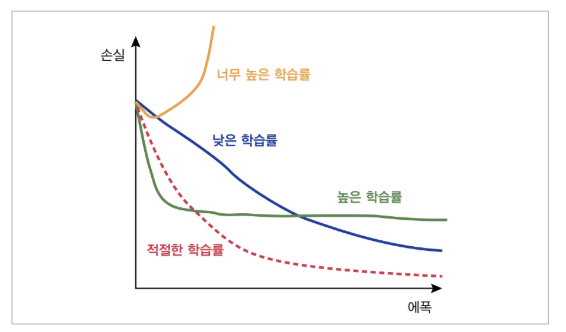
따라서 실질적으로 Learning Rate를 크게 설정하고 점차 줄여가는 방안으로서 학습하였었다.
Pytorch에서는 이러한 Learning Rate를 여러번의 Trainning이 아닌 학습률을 점차 떨어뜨리는 방법으로서 구현하였다.
torch.optim.lr_scheduler.StepLR(optimizer, step_size, gamma=0.1, last_epoch=-1)
- optimizer(Optimizer): Optimizer
- step_size(int): Period of learning rate decay
- gamma(float): Multiplicative factor of learning rate decay
- last_epoch(int): The index of last epoch. Default: -1 정해진 Step_size마다 Learning Rate에 gamma를 곱하여 Learning Rate를 감소
torch.optim.lr_scheduler.MultiStepLR(optimizer, milestones, gamma=0.1, last_epoch=-1)
- optimizer(Optimizer): Optimizer
- milestones (list) – List of epoch indices. Must be increasing.
- gamma(float): Multiplicative factor of learning rate decay
- last_epoch(int): The index of last epoch. Default: -1 Step_size를 List로서 받아서 원하는 지점마다 학습률을 감소
torch.optim.lr_scheduler.ExponentialLR(optimizer, gamma, last_epoch=-1)
- optimizer(Optimizer): Optimizer
- gamma(float): Multiplicative factor of learning rate decay
- last_epoch(int): The index of last epoch. Default: -1 매 Epoch마다 Learning Rate에 gamma를 곱하여 Learning Rate를 감소
ExponentialLR Model
1) CNN Model
1
2
3
4
5
6
7
8
9
10
11
12
13
14
15
16
17
18
19
20
21
22
23
24
class CNN(nn.Module):
    def __init__(self):
        super(CNN,self).__init__()
        self.layer = nn.Sequential(
            nn.Conv2d(1,16,3,padding=1),  # 28 x 28
            nn.ReLU(),
            nn.Conv2d(16,32,3,padding=1), # 28 x 28
            nn.ReLU(),
            nn.MaxPool2d(2,2),            # 14 x 14
            nn.Conv2d(32,64,3,padding=1), # 14 x 14
            nn.ReLU(),
            nn.MaxPool2d(2,2)             #  7 x 7
        )
        self.fc_layer = nn.Sequential(
            nn.Linear(64*7*7,100),
            nn.ReLU(),
            nn.Linear(100,10)
        )

    def forward(self,x):
        out = self.layer(x)
        out = out.view(batch_size,-1)
        out = self.fc_layer(out)
        return out
2) Loss func & Optimizer
1
2
3
4
5
6
7
8
9
10
11
12
13
14
15
16
17
18
19
20
from torch.optim import lr_scheduler

device = torch.device("cuda:0" if torch.cuda.is_available() else "cpu")
print(device)

model = CNN().to(device)
loss_func = nn.CrossEntropyLoss()
optimizer = torch.optim.SGD(model.parameters(), lr=learning_rate)

# 지정한 스텝 단위로 학습률에 감마를 곱해 학습률을 감소시킵니다.
#scheduler = lr_scheduler.StepLR(optimizer, step_size=1, gamma= 0.99)

# 지정한 스텝 지점(예시에서는 10,30,80)마다 학습률에 감마를 곱해줍니다.
#scheduler = lr_scheduler.MultiStepLR(optimizer, milestones=[10,30,80], gamma= 0.1)

# 매 epoch마다 학습률에 감마를 곱해줍니다.
scheduler = lr_scheduler.ExponentialLR(optimizer, gamma= 0.99)

print(dir(scheduler))
print(dir(optimizer))
cuda:0
['__class__', '__delattr__', '__dict__', '__dir__', '__doc__', '__eq__', '__format__', '__ge__', '__getattribute__', '__gt__', '__hash__', '__init__', '__init_subclass__', '__le__', '__lt__', '__module__', '__ne__', '__new__', '__reduce__', '__reduce_ex__', '__repr__', '__setattr__', '__sizeof__', '__str__', '__subclasshook__', '__weakref__', '_step_count', 'base_lrs', 'gamma', 'get_lr', 'last_epoch', 'load_state_dict', 'optimizer', 'state_dict', 'step']
['__class__', '__delattr__', '__dict__', '__dir__', '__doc__', '__eq__', '__format__', '__ge__', '__getattribute__', '__getstate__', '__gt__', '__hash__', '__init__', '__init_subclass__', '__le__', '__lt__', '__module__', '__ne__', '__new__', '__reduce__', '__reduce_ex__', '__repr__', '__setattr__', '__setstate__', '__sizeof__', '__str__', '__subclasshook__', '__weakref__', '_step_count', 'add_param_group', 'defaults', 'load_state_dict', 'param_groups', 'state', 'state_dict', 'step', 'zero_grad']
3) Train
1
2
3
4
5
6
7
8
9
10
11
12
13
14
15
16
17
for i in range(num_epoch):
    scheduler.step()
    for j,[image,label] in enumerate(train_loader):
        x = image.to(device)
        y_= label.to(device)

        optimizer.zero_grad()
        output = model.forward(x)
        loss = loss_func(output,y_)
        loss.backward()


    if i % 10 == 0:
        print(loss)

    #print("Epoch: {}, Learning Rate: {}".format(i,scheduler.get_lr()))
    print("Epoch: {}, Learning Rate: {}".format(i,scheduler.optimizer.state_dict()['param_groups'][0]['lr']))
tensor(2.2967, device='cuda:0', grad_fn=<NllLossBackward>)
Epoch: 0, Learning Rate: 0.00017323173233307898
Epoch: 1, Learning Rate: 0.00017149941413663328
Epoch: 2, Learning Rate: 0.00016978442727122456
Epoch: 3, Learning Rate: 0.00016808656801003963
Epoch: 4, Learning Rate: 0.00016640570538584143
Epoch: 5, Learning Rate: 0.000164741650223732
Epoch: 6, Learning Rate: 0.0001630942424526438
Epoch: 7, Learning Rate: 0.00016146330744959414
Epoch: 8, Learning Rate: 0.00015984867059160024
Epoch: 9, Learning Rate: 0.00015825020091142505
4) Test
1
2
3
4
5
6
7
8
9
10
11
12
13
14
15
correct = 0
total = 0

with torch.no_grad():
  for image,label in test_loader:
      x = image.to(device)
      y_= label.to(device)

      output = model.forward(x)
      _,output_index = torch.max(output,1)

      total += label.size(0)
      correct += (output_index == y_).sum().float()

  print("Accuracy of Test Data: {}".format(100*correct/total))
tensor(2.4497, grad_fn=<AddBackward0>)
tensor(1.0887, grad_fn=<AddBackward0>)
tensor(0.6670, grad_fn=<AddBackward0>)

...

tensor(0.0032, grad_fn=<AddBackward0>)
tensor(0.0021, grad_fn=<AddBackward0>)
tensor(0.0016, grad_fn=<AddBackward0>)
Normalization
정규화의 종류로는 크게 2가지가 존재한다.
- 표준 정규화: \(\hat{x} = \frac{x - m}{\alpha}\)
- 최소극대화 정규화: \(x = (x - min(x))/(max(x) - min(x))\)
정규화의 문제로는 너무 작거나 큰 이상치가 있는 경우에는 오히려 학습에 방해가 되는 경우도 발생한다.
아래 그림은 정규화를 하였을때 장점중 하나를 표현한 것이다.

위의 그림과 같이 데이터의 각 요소별 범위가 같은 비율로서 Update함으로써 더 빠른 Update를 기대할 수 있다.
Normalization Model
1) 데이터 정규화
transforms.Normalization을 통화여 정규화가 가능하다.
각각의 Parameter가 여러개인 것은 들어오는 Input Image의 Channel을 모르기 때문이다.
1
2
3
4
5
6
7
8
9
10
11
12
13
14
15
16
17
mnist_train = dset.MNIST("./", train=True,
                         transform=transforms.Compose([
                             transforms.ToTensor(),
                             transforms.Normalize(mean=(0.1307,), std=(0.3081,))
                         ]),
                         target_transform=None,
                         download=True)
mnist_test = dset.MNIST("./", train=False,
                        transform=transforms.Compose([
                             transforms.ToTensor(),
                             transforms.Normalize(mean=(0.1307,), std=(0.3081,))
                        ]),
                        target_transform=None,
                        download=True)

train_loader = torch.utils.data.DataLoader(mnist_train,batch_size=batch_size, shuffle=True,num_workers=2,drop_last=True)
test_loader = torch.utils.data.DataLoader(mnist_test,batch_size=batch_size, shuffle=False,num_workers=2,drop_last=True)
2) CNN Model
1
2
3
4
5
6
7
8
9
10
11
12
13
14
15
16
17
18
19
20
21
22
23
24
class CNN(nn.Module):
    def __init__(self):
        super(CNN,self).__init__()
        self.layer = nn.Sequential(
            nn.Conv2d(1,16,3,padding=1),  # 28 x 28
            nn.ReLU(),
            nn.Conv2d(16,32,3,padding=1), # 28 x 28
            nn.ReLU(),
            nn.MaxPool2d(2,2),            # 14 x 14
            nn.Conv2d(32,64,3,padding=1), # 14 x 14
            nn.ReLU(),
            nn.MaxPool2d(2,2)             #  7 x 7
        )
        self.fc_layer = nn.Sequential(
            nn.Linear(64*7*7,100),
            nn.ReLU(),
            nn.Linear(100,10)
        )

    def forward(self,x):
        out = self.layer(x)
        out = out.view(batch_size,-1)
        out = self.fc_layer(out)
        return out
3) Loss func & Optimizer
1
2
3
4
5
6
device = torch.device("cuda:0" if torch.cuda.is_available() else "cpu")
print(device)

model = CNN().to(device)
loss_func = nn.CrossEntropyLoss()
optimizer = torch.optim.SGD(model.parameters(), lr=learning_rate)
4) Train
1
2
3
4
5
6
7
8
9
10
11
12
13
for i in range(num_epoch):
    for j,[image,label] in enumerate(train_loader):
        x = image.to(device)
        y_= label.to(device)

        optimizer.zero_grad()
        output = model.forward(x)
        loss = loss_func(output,y_)
        loss.backward()
        optimizer.step()

    if i % 10 == 0:
        print(loss)
5) Test
1
2
3
4
5
6
7
8
9
10
11
12
13
14
15
correct = 0
total = 0

with torch.no_grad():
  for image,label in test_loader:
      x = image.to(device)
      y_= label.to(device)

      output = model.forward(x)
      _,output_index = torch.max(output,1)

      total += label.size(0)
      correct += (output_index == y_).sum().float()

  print("Accuracy of Test Data: {}".format(100*correct/total))
Accuracy of Test Data: 34.0044059753418
Batch Normalization
배치 정규화는 활성함수의 활성화값 또는 출력값을 정규화 하는 작업을 의미한다. 이는 데이터 분포가 치우치는 현상을 해결함으로써 가중치가 엉뚱한 방향으로 갱신될 문제를 해결할 수 있다.
배치 정규화의 과정은 아래와 같은 그림으로 나타낼 수 있다.
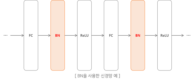
위의 그림으로서 데이터의 분포가 평균이 0, 분산이 1이 되도록 정규화를 한다.
수식으로는 아래와 같이 나타낼 수 있다.
$$ \mu_B \leftarrow \frac{1}{m}\sum_{i=1}^m x_i$$
$$ \sigma_B^2 \leftarrow \frac{1}{m}\sum_{i=1}^m (x_i-\mu_B)^2$$
$$ \hat{x_i} \leftarrow \frac{x_i-\mu_B}{\sqrt{\sigma_B^2 + \varepsilon}}$$
$$ B = {x_1, x_2, ... , x_m} $$
위의 식에서 알 수 있듯이 m개의 입력 데이터의 집합에 대해 평균 \(\mu_B\)와 분산\(\sigma_B^2\)를 구한다.
그리고 입력 데이터를 평균이 0, 분산이 1이 되게 정규화를 실시한다.
\(\varepsilon\)는 매우 작은 값으로서 \(\frac{x_i-\mu_B}{\sqrt{\sigma_B^2 + \varepsilon}}\)의 값이 inf가 되는 것을 방지한다.
Pytorch에서는 nn.BatchNorm()으로서 구성한다.
또한 DropOut기법과 똑같이 Train에서는 BatchNormalization을 실시하고 평가할때는 model.eval()을 통하여 BatchNormalization을 실시하지 않는다.
위에서도 알 수 있듯이 Normalization은 Train Dataset과 Test Dataset을 똑같이 Normalization을 시켜서 Update하는 거라면 Batch Normalization은 같은 Batch Data끼리의 Normalization을 통하여 Update하는 것 이다.
Batch Normalization Model
1) 데이터 Batch
1
2
3
4
5
mnist_train = dset.MNIST("./", train=True, transform=transforms.ToTensor(), target_transform=None, download=True)
mnist_test = dset.MNIST("./", train=False, transform=transforms.ToTensor(), target_transform=None, download=True)

train_loader = torch.utils.data.DataLoader(mnist_train,batch_size=batch_size, shuffle=True,num_workers=2,drop_last=True)
test_loader = torch.utils.data.DataLoader(mnist_test,batch_size=batch_size, shuffle=False,num_workers=2,drop_last=True)
2) CNN Model
1
2
3
4
5
6
7
8
9
10
11
12
13
14
15
16
17
18
19
20
21
22
23
24
25
26
27
28
29
30
31
32
33
# 입력 데이터를 정규화하는것처럼 연산을 통과한 결과값을 정규화할 수 있습니다.
# 그 다양한 방법중에 대표적인것이 바로 Batch Normalization이고 이는 컨볼루션 연산처럼 모델에 한 층으로 구현할 수 있습니다.
# https://pytorch.org/docs/stable/nn.html?highlight=batchnorm#torch.nn.BatchNorm2d
# nn.BatchNorm2d(x)에서 x는 입력으로 들어오는 채널의 개수입니다.

class CNN(nn.Module):
    def __init__(self):
        super(CNN,self).__init__()
        self.layer = nn.Sequential(
            nn.Conv2d(1,16,3,padding=1),  # 28 x 28
            nn.BatchNorm2d(16),
            nn.ReLU(),
            nn.Conv2d(16,32,3,padding=1), # 28 x 28
            nn.BatchNorm2d(32),
            nn.ReLU(),
            nn.MaxPool2d(2,2),            # 14 x 14
            nn.Conv2d(32,64,3,padding=1), # 14 x 14
            nn.BatchNorm2d(64),
            nn.ReLU(),
            nn.MaxPool2d(2,2)             #  7 x 7
        )
        self.fc_layer = nn.Sequential(
            nn.Linear(64*7*7,100),
            nn.BatchNorm1d(100),
            nn.ReLU(),
            nn.Linear(100,10)
        )

    def forward(self,x):
        out = self.layer(x)
        out = out.view(batch_size,-1)
        out = self.fc_layer(out)
        return out
3) Loss func & Optimizer
1
2
3
4
5
6
device = torch.device("cuda:0" if torch.cuda.is_available() else "cpu")
print(device)

model = CNN().to(device)
loss_func = nn.CrossEntropyLoss()
optimizer = torch.optim.SGD(model.parameters(), lr=learning_rate)
4) Train
1
2
3
4
5
6
7
8
9
10
11
12
13
for i in range(num_epoch):
    for j,[image,label] in enumerate(train_loader):
        x = image.to(device)
        y_= label.to(device)

        optimizer.zero_grad()
        output = model.forward(x)
        loss = loss_func(output,y_)
        loss.backward()
        optimizer.step()

    if i % 10 == 0:
        print(loss)
5) Test
1
2
3
4
5
6
7
8
9
10
11
12
13
14
15
16
17
correct = 0
total = 0

# 배치정규화나 드롭아웃은 학습할때와 테스트 할때 다르게 동작하기 때문에 모델을 evaluation 모드로 바꿔서 테스트해야합니다.
model.eval()
with torch.no_grad():
  for image,label in test_loader:
      x = image.to(device)
      y_= label.to(device)

      output = model.forward(x)
      _,output_index = torch.max(output,1)

      total += label.size(0)
      correct += (output_index == y_).sum().float()

  print("Accuracy of Test Data: {}".format(100*correct/total))
Accuracy of Test Data: 91.85697174072266
다양한 Optimazation
NeuralNetwork (3) Optimazation2에 Optimizer가 고려해야 하는 사항과 다양한 Optimizer를 소개하였다.
Pytorch에서는 torch.optim에서 이러한 종류를 구현하여서 제공하고 있다.
SGD
torch.optim.SGD(params, lr=required parameter, momentum=0, dampening=0, weight_decay=0, nesterov=False)
AdaGrad
torch.optim.Adagrad(params, lr=0.01, lr_decay=0, weight_decay=0, initial_accumulator_value=0)
RMS Prop
torch.optim.RMSprop(params, lr=0.01, alpha=0.99, eps=1e-08, weight_decay=0, momentum=0, centered=False)
Adam
torch.optim.Adam(params, lr=0.001, betas=(0.9, 0.999), eps=1e-08, weight_decay=0, amsgrad=False)
참조: 원본코드
참조: 파이토치 첫걸음
코드에 문제가 있거나 궁금한 점이 있으면 wjddyd66@naver.com으로 Mail을 남겨주세요.
Leave a comment