DataAnalysis-분류분석

분류(Classfication)

소속 집단을 알고 있는 데이터를 이용하여 모형을 만들어서 소속집단을 모르는 데이터들의 집단을 결정하는 기법
Supervised Learning.

1. 로지스틱 회귀(Logistic regression)
2. 의사결정 나무(Decision Tree)
3. 랜덤 포레스트(Random Forest)
4. 나이브베이즈 분류(Naive Bayes Classification)
5. SVM(Support Vector Machine)
6. K-NN Classfication

위에대한 자세한 내용은 아래 링크 참조
분류분석 자세한 내용

공통사항

많은 분류분석을 비교하기 전에 공통적으로 사용하는 것을 Method로서 선언하였다.
Data 는 Iris Data중 Sepal length, Sepal width를 사용하였다.
from sklearn.model_selection import train_test_split를 활용하여 전체 Data중에서 30%는 Test, 70%는 Train으로서 사용하였다.

#Iris Data 불러오기
iris = datasets.load_iris()
X = iris.data[:, :2]
Y = iris.target
#Train, Test DataSet분리
train_x, test_x, train_y ,test_y = train_test_split(X,Y, test_size = 0.3, random_state=0)

정확도를 측정하는 Method는 Parameter로서 예상값, 실제값, Train or Test인지 알려주는 String parameter을 받아 정확도를 측정하게 된다.

#정확도 측정 Method
def accuracy(X,Y,S):
    total = len(X)
    count = 0
    for i in range(1,len(X)):
      if(X[i] == Y[i]):
        count = count+1
    print(S,'정확도는 ',round(count/total,4)*100,'% 입니다')

시각화를 하는 Method는 실제 Data의 분포와 이것을 어떻게 분리했는지를 나타내주는 Method이다.
아래 코드는 다음을 참조하여서 작성하였다.
시각화 코드 참조 사이트

#시각화 Method
def visualization(model):
    x_min, x_max = X[:, 0].min() - .5, X[:, 0].max() + .5
    y_min, y_max = X[:, 1].min() - .5, X[:, 1].max() + .5
    h = .02  # step size in the mesh
    xx, yy = np.meshgrid(np.arange(x_min, x_max, h), np.arange(y_min, y_max, h))
    Z = model.predict(np.c_[xx.ravel(), yy.ravel()])

    # Put the result into a color plot
    Z = Z.reshape(xx.shape)
    plt.figure(1, figsize=(4, 3))
    plt.pcolormesh(xx, yy, Z, cmap=plt.cm.Paired)

    # Plot also the training points
    plt.scatter(X[:, 0], X[:, 1], c=Y, edgecolors='k', cmap=plt.cm.Paired)
    plt.xlabel('Sepal length')
    plt.ylabel('Sepal width')

    plt.xlim(xx.min(), xx.max())
    plt.ylim(yy.min(), yy.max())
    plt.xticks(())
    plt.yticks(())

    plt.show()

로지스틱 회귀(Logistic regression)

로지스틱 회귀는 다음과 같은 code를 import하여 사용할 수 있다.

from sklearn.linear_model import LogisticRegression

로지스틱 회귀 Parameter 참조 사이트

로지스틱 회귀 구현

#Logistic Regression
logreg = LogisticRegression(C=1e5, solver='lbfgs', multi_class='multinomial')

# Create an instance of Logistic Regression Classifier and fit the data.
logreg.fit(train_x, train_y)
#Traing 정확도
accuracy(train_y,logreg.predict(train_x),'Train ')
#Test 정확도
accuracy(test_y,logreg.predict(test_x),'Test ')
#시각화
visualization(logreg)

Train 정확도는 82.86 % 입니다
Test 정확도는 80.0 % 입니다
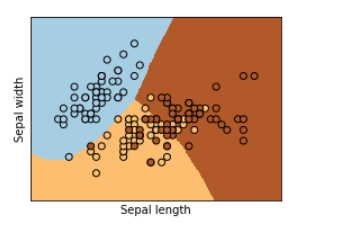
로지스틱 회귀 시각화

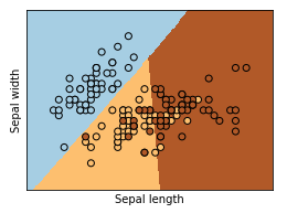
의사결정 나무(Decision Tree)

의사결정 나무는 다음과 같은 code를 import하여 사용할 수 있다.

from sklearn import tree

의사결정 나무 Parameter 참조 사이트

의사결정 나무 구현

#Decision Tree
import pydotplus
from sklearn import tree

DecisionTree = tree.DecisionTreeClassifier(criterion= "entropy", max_depth=3)
DecisionTree.fit(train_x, train_y)

#Traing 정확도
accuracy(train_y,DecisionTree.predict(train_x),'Train ')
#Test 정확도
accuracy(test_y,DecisionTree.predict(test_x),'Test ')

#시각화
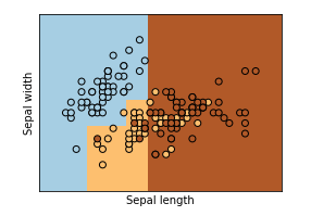
visualization(DecisionTree)

Train 정확도는 81.89999999999999 % 입니다
Test 정확도는 66.67 % 입니다
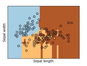
의사결정 나무 시각화1

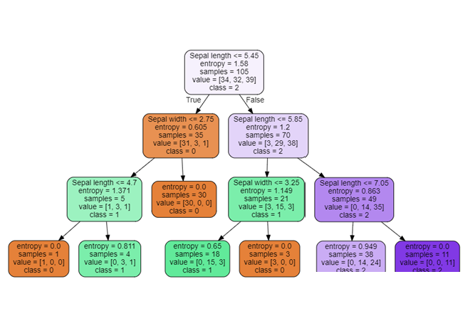
의사결정 나무 시각화2

#Decision Treee 시각화
from matplotlib.pyplot import imread
import graphviz

label_names=['Sepal length','Sepal width']
dot_data = tree.export_graphviz(DecisionTree, feature_names=label_names,
                                out_file='tree.dot',class_names=["0","1","2"], filled=True, rounded=True)

with open("tree.dot") as f:
    dot_graph = f.read()
display(graphviz.Source(dot_graph))

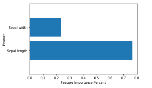
의사결정 나무 중요도 시각화

#Decision Treee 중요도 시각화
def plot_feature_importances(model):
    plt.barh(range(2), model.feature_importances_, align='center')
    plt.yticks(np.arange(2), ['Sepal length','Sepal width'])
    plt.xlabel("Feature Importance Percent")
    plt.ylabel("Feature")
    plt.ylim(-1, 2)

plot_feature_importances(DecisionTree)

랜덤포레스트(Random Forest)

랜덤포레스트는 다음과 같은 code를 import하여 사용할 수 있다.

from sklearn.ensemble import RandomForestClassifier

랜덤포레스트 Parameter 참조 사이트

랜덤포레스트 구현

#Random Forest
from sklearn.ensemble import RandomForestClassifier

RandomForest = RandomForestClassifier(criterion = "entropy", n_estimators=10)
RandomForest.fit(train_x, train_y)

#Traing 정확도
accuracy(train_y,RandomForest.predict(train_x),'Train ')
#Test 정확도
accuracy(test_y,RandomForest.predict(test_x),'Test ')
#시각화
visualization(RandomForest)

Train 정확도는 91.43 % 입니다
Test 정확도는 66.67 % 입니다
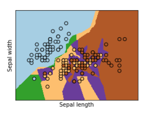
랜덤포레스트 시각화

나이브베이즈 분류(Naive Bayes Classification)

나이브베이즈 분류는 다음과 같은 code를 import하여 사용할 수 있다.

from sklearn.naive_bayes import GaussianNB

나이브베이즈 Parameter 참조 사이트

나이브베이즈 분류 구현

#Naive Bayes Classification
from sklearn.naive_bayes import GaussianNB
NaiveBayes = GaussianNB().fit(train_x, train_y)
#Traing 정확도
accuracy(train_y,NaiveBayes.predict(train_x),'Train ')
#Test 정확도
accuracy(test_y,NaiveBayes.predict(test_x),'Test ')
#시각화
visualization(NaiveBayes)

Train 정확도는 80.0 % 입니다
Test 정확도는 80.0 % 입니다
나이브베이즈 분류 시각화

K-NN Classfication

K-NN Classfication는 다음과 같은 code를 import하여 사용할 수 있다.

from sklearn.neighbors import KNeighborsRegressor

K-NN Parameter 참조 사이트

K-NN Classfication 구현

#K-NN
from sklearn.neighbors import KNeighborsRegressor
KNN = KNeighborsRegressor(n_neighbors = 2, n_jobs = -1)
# n_jobs = -1 : "직접 판단하라는 의미"
KNN.fit(train_x, train_y)
#Traing 정확도
accuracy(train_y,KNN.predict(train_x),'Train ')
#Test 정확도
accuracy(test_y,KNN.predict(test_x),'Test ')
#시각화
visualization(KNN)

Train 정확도는 73.33 % 입니다
Test 정확도는 53.33 % 입니다
K-NN Classfication 시각화

SVM(Support Vector Machine)

SVM는 다음과 같은 code를 import하여 사용할 수 있다.

from sklearn import svm

SVM Parameter 참조 사이트

SVM 구현

#SVM
from sklearn import svm
SVM = svm.LinearSVC(C=10)
SVM.fit(train_x, train_y)

#Traing 정확도
accuracy(train_y,SVM.predict(train_x),'Train ')
#Test 정확도
accuracy(test_y,SVM.predict(test_x),'Test ')
#시각화
visualization(SVM)

Train 정확도는 80.95 % 입니다
Test 정확도는 80.0 % 입니다
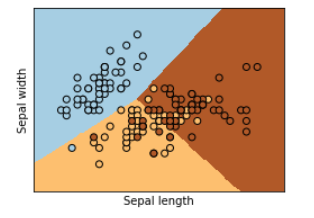
SVM 시각화

최종결과

방법	정확도
Logistic Regression	Train: 82.86% Test: 80.00%
Decision Tree	Train: 81.89% Test: 66.67%
Random Forest	Train: 91.43% Test: 66.67%
Naive Bayes Classification	Train: 80.00% Test: 80.00%
K-NN	Train: 73.33% Test: 53.33%
SVM	Train: 80.95% Test: 80.00%

위의 결과표를 참조하면 SVM, Logistic Regression, Naive Bayes Classification이 가장 적절한 Model이라는 것을 판단할 수 있다.
하지만 위에서의 Code는 조정 가능한 Parameter를 바꿔가면서 비교한 것이 아니다.
실제 Model을 만들고 적용할 떄는 조정 가능한 Parameter를 조정해가면서 최적의 Model을 찾는 것이 필요하다.

---

잠조: 원본코드
코드에 문제가 있거나 궁금한 점이 있으면 wjddyd66@naver.com으로 Mail을 남겨주세요.