
DataAnalysis-회귀분석
회귀분석
회귀분석은 상관분석과 더불어 널리 쓰이는 통계적 방법이다. 상관분석이 상관관계를 알아보기 위함이라면 회귀분석의 경우 인과관계를 파악하는 분석 방법이다.
회귀분석의 대한 자세한 내용은 아래 링크 참조
회귀분석 자세한 내용
회귀 분석 방법
Python으로 회귀분석은 크게 4가지가 가능하다.
- make regression
- LinearRegression Model
- ols
- scipy.stats.linregress
MakeRegression
실제로 운영하기에는 현실적으로 무리가 있는 방법이다.
이렇게 사용 가능하다는 것만 알아두자.
1
2
3
4
5
6
7
8
9
10
11
12
13
14
15
16
17
18
19
20
21
#Make Regression
print("Make Regression")
from sklearn.datasets import make_regression

np.random.seed(12)
x, y, coef = make_regression(n_samples = 50, n_features = 1, bias = 100, coef = True)
# n_features : 독립변수. bias : 절편 (디폴트=0.0), coef : 기울기
print(x[[range(1,5)]])
print(y[[range(1,5)]])
print(coef)
# 표본데이터(x) 50개와 그에따른 y값 50개 반환되었다.
y_pred  = 100 + 89.47430739278907 * -1.70073563
# y_pred : 예측에 의한 y값
#bias: 89.47430739278907
#weight:-1.70073563
print(y)
# 수식에 의해 예측한 값 = -52.17214255248879
# 실제값 = -52.17214291
# make regression을 이용해 x를 입력하면 수식에 의해 예측된 y값을 도출해낼 수 있다.
# 실제로 운영하기에는 현실적으로 다소 무리가 있다.
# 있다는 것만 알고 넘어가자.
Make Regression
[[-0.67794537]
 [ 0.31866529]
 [ 0.13884618]
 [ 0.53513589]]
[ 39.34130801 128.51235594 112.42316554 147.88091341]
89.47430739278907
[ -52.17214291   39.34130801  128.51235594  112.42316554  147.88091341
   96.49178624  103.16885304   36.12820309   89.71761789  190.59412103
  300.58509445  100.45874176    7.88349776   42.07157936  142.32007968
   -8.72638684   77.28210847   65.60976235  147.18272498  142.27276227
   18.23219105  144.90467678   39.0298914   -98.0364801    89.07073235
   48.8313381   220.10640661   -3.28558253   47.63352619 -181.61291334
  119.23482409  -50.47399897   27.79585534  208.24569942  198.05991459
   46.51020834   10.77587732   52.72138937   89.24271248  106.55417864
   90.52804266  167.38693344  121.69210605  -98.50187763  -59.98849467
  356.95405132  219.52258382  -37.31812896  157.33165682   69.79389882]
LinearRegression
sklearn에 있는 패키지를 사용하는 방법이다.
아래 코드를 활용하여 LinearRegression을 import하여 사용할 수 있다.
1
from sklearn.linear_model import LinearRegression
LinearRegression은 n_jobs: cpu에 따라 병렬로 처리할 수 있게 해주는 Option이 존재한다.
LinearRegressio을 활용하여 Model만들기
1
2
3
4
5
6
7
8
9
10
11
12
13
14
#LinearRegression
x1 = x
y1 = y
from sklearn.linear_model import LinearRegression
model = LinearRegression(fit_intercept=True, n_jobs=None)
#n_jobs: cpu에 따라 병렬로 처리할 수 있게 해주는 Option

print(model)
fit_model = model.fit(x1, y1)

print("기울기: ", fit_model.coef_)
print("절편: ", fit_model.intercept_)
y_new = fit_model.predict(x1)
print(y_new)
LinearRegression(copy_X=True, fit_intercept=True, n_jobs=None, normalize=False)
기울기:  [89.47430739]
절편:  100.0
[ -52.17214291   39.34130801  128.51235594  112.42316554  147.88091341
   96.49178624  103.16885304   36.12820309   89.71761789  190.59412103
  300.58509445  100.45874176    7.88349776   42.07157936  142.32007968
   -8.72638684   77.28210847   65.60976235  147.18272498  142.27276227
   18.23219105  144.90467678   39.0298914   -98.0364801    89.07073235
   48.8313381   220.10640661   -3.28558253   47.63352619 -181.61291334
  119.23482409  -50.47399897   27.79585534  208.24569942  198.05991459
   46.51020834   10.77587732   52.72138937   89.24271248  106.55417864
   90.52804266  167.38693344  121.69210605  -98.50187763  -59.98849467
  356.95405132  219.52258382  -37.31812896  157.33165682   69.79389882]
Linear Regression을 활용하여 새로운 값 예측
1
2
3
4
5
#Linear Regression을 활용하여 새로운 값 예측
x_new, _, _ = make_regression(n_samples = 5, n_features = 1, bias = 100, coef = True)
print(x_new)
y_pred2 = fit_model.predict(x_new)
print(y_pred2)
[[-0.5314769 ]
 [ 0.86721724]
 [-1.25494726]
 [ 0.93016889]
 [-1.63412849]]
[ 52.44647266 177.59366163 -12.28553693 183.2262176  -46.21251453]
ols
statsmodels 에 있는 패키지를 사용하는 방법이다.
아래 코드를 활용하여 ols을 import하여 사용할 수 있다.
1
import statsmodels.formula.api as smf
ols Model만들기
1
2
3
4
5
6
7
8
9
10
x1 = x.flatten()
#flatten(): 차원 축소
print(x1.shape)
print(y1.shape)
data = np.array([x1, y1])
df = pd.DataFrame(data.T)
df.columns = ["x1", "y1"]
print(df.head(3))
model = smf.ols(formula = "y1 ~ x1", data = df).fit()
print(model.summary())
(50,)
(50,)
         x1          y1
0 -1.700736  -52.172143
1 -0.677945   39.341308
2  0.318665  128.512356
                            OLS Regression Results
==============================================================================
Dep. Variable:                     y1   R-squared:                       1.000
Model:                            OLS   Adj. R-squared:                  1.000
Method:                 Least Squares   F-statistic:                 1.905e+32
Date:                Tue, 30 Jul 2019   Prob (F-statistic):               0.00
Time:                        21:12:20   Log-Likelihood:                 1460.6
No. Observations:                  50   AIC:                            -2917.
Df Residuals:                      48   BIC:                            -2913.
Df Model:                           1
Covariance Type:            nonrobust
==============================================================================
                 coef    std err          t      P>|t|      [0.025      0.975]
------------------------------------------------------------------------------
Intercept    100.0000   7.33e-15   1.36e+16      0.000     100.000     100.000
x1            89.4743   6.48e-15   1.38e+16      0.000      89.474      89.474
==============================================================================
Omnibus:                        7.616   Durbin-Watson:                   1.798
Prob(Omnibus):                  0.022   Jarque-Bera (JB):                8.746
Skew:                           0.516   Prob(JB):                       0.0126
Kurtosis:                       4.770   Cond. No.                         1.26
==============================================================================
Model 해석
1
2
3
4
5
6
print("기울기: ", model.params['x1'])
print("절편: ", model.params['Intercept'])
print("pvalue",model.pvalues)
#pvalue(0) <0.05 이므로 통계적으로 유의하다.
print("설명력",model.rsquared)
#설명력은 100%로 설명력이 높다.
기울기:  89.47430739278903
절편:  99.99999999999999
pvalue Intercept    0.0
x1           0.0
dtype: float64
설명력 1.0
Iris Data를 활용하여 단순회귀 분석과 다중회귀 분석을 하는 예제이다.
단순 회귀 분석은 상관계수에 따른 결과 확인을 한다.
단순 회귀 분석(1) 상관계수 낮은 변수 사용
1
2
3
4
5
6
7
8
9
10
11
12
13
14
15
#Iris를 활용한 단순 회귀 분석
#상관관계에 따른 결과 확인
import seaborn as sns
print("\n#1. 단순회귀분석")
iris = sns.load_dataset("iris")
print(iris.head(3))
print('상관계수',iris.corr())
#sepal_length ~ sepal_width 의 상관계수 = -0.117570

result = smf.ols("sepal_length ~ sepal_width", data = iris).fit()
print(result.summary())
print("결정 계수: ", result.rsquared)
#0.013822654141080859 => 설명력이 낮다.
print("p값: ", result.pvalues)
print("실제값: ", iris.sepal_length[0], "예측값: ", result.predict()[0])
#1. 단순회귀분석
   sepal_length  sepal_width  petal_length  petal_width species
0           5.1          3.5           1.4          0.2  setosa
1           4.9          3.0           1.4          0.2  setosa
2           4.7          3.2           1.3          0.2  setosa
상관계수               sepal_length  sepal_width  petal_length  petal_width
sepal_length      1.000000    -0.117570      0.871754     0.817941
sepal_width      -0.117570     1.000000     -0.428440    -0.366126
petal_length      0.871754    -0.428440      1.000000     0.962865
petal_width       0.817941    -0.366126      0.962865     1.000000
                            OLS Regression Results
==============================================================================
Dep. Variable:           sepal_length   R-squared:                       0.014
Model:                            OLS   Adj. R-squared:                  0.007
Method:                 Least Squares   F-statistic:                     2.074
Date:                Tue, 30 Jul 2019   Prob (F-statistic):              0.152
Time:                        21:12:20   Log-Likelihood:                -183.00
No. Observations:                 150   AIC:                             370.0
Df Residuals:                     148   BIC:                             376.0
Df Model:                           1
Covariance Type:            nonrobust
===============================================================================
                  coef    std err          t      P>|t|      [0.025      0.975]
-------------------------------------------------------------------------------
Intercept       6.5262      0.479     13.628      0.000       5.580       7.473
sepal_width    -0.2234      0.155     -1.440      0.152      -0.530       0.083
==============================================================================
Omnibus:                        4.389   Durbin-Watson:                   0.952
Prob(Omnibus):                  0.111   Jarque-Bera (JB):                4.237
Skew:                           0.360   Prob(JB):                        0.120
Kurtosis:                       2.600   Cond. No.                         24.2
==============================================================================
결정 계수:  0.013822654141080859
p값:  Intercept      6.469702e-28
sepal_width    1.518983e-01
dtype: float64
실제값:  5.1 예측값:  5.744458836939834
단순 회귀 분석(2) 상관계수 높은 변수 사용
1
2
3
4
5
6
7
8
result2 = smf.ols("sepal_length ~ petal_length", data = iris).fit()
#sepal_length ~ petal_length 의 상관계수 = 0.871754
print(result2.summary())
print("결정 계수: ", result2.rsquared)
#75% 이므로 충분히 설명력을 가진다.
print("p값: ", result2.pvalues)
#pvalue(2.426713e-100) < 0.05 이므로 통계적으로 유의하다.
print("실제값: ", iris.sepal_length[0], "예측값: ", result2.predict()[0])
                            OLS Regression Results
==============================================================================
Dep. Variable:           sepal_length   R-squared:                       0.760
Model:                            OLS   Adj. R-squared:                  0.758
Method:                 Least Squares   F-statistic:                     468.6
Date:                Tue, 30 Jul 2019   Prob (F-statistic):           1.04e-47
Time:                        21:12:20   Log-Likelihood:                -77.020
No. Observations:                 150   AIC:                             158.0
Df Residuals:                     148   BIC:                             164.1
Df Model:                           1
Covariance Type:            nonrobust
================================================================================
                   coef    std err          t      P>|t|      [0.025      0.975]
--------------------------------------------------------------------------------
Intercept        4.3066      0.078     54.939      0.000       4.152       4.462
petal_length     0.4089      0.019     21.646      0.000       0.372       0.446
==============================================================================
Omnibus:                        0.207   Durbin-Watson:                   1.867
Prob(Omnibus):                  0.902   Jarque-Bera (JB):                0.346
Skew:                           0.069   Prob(JB):                        0.841
Kurtosis:                       2.809   Cond. No.                         10.3
==============================================================================

결정 계수:  0.7599546457725151
p값:  Intercept       2.426713e-100
petal_length     1.038667e-47
dtype: float64
실제값:  5.1 예측값:  4.879094603339241
다중 회귀 분석 Model 1
1
2
3
4
5
6
7
8
9
10
11
#Iris를 활용한 다중 회귀 분석
print("\n#2. 다중회귀분석")
# 다중회귀분석 formula = "y ~ x1 + x2 + ..."
result3 = smf.ols(formula = "sepal_length ~ petal_length + petal_width", data = iris).fit()
print(result3.summary())
print("결정 계수: ", result3.rsquared)
print("p값: ", result3.pvalues)
'''
결정 계수:  0.7662612975425306 => 충분한 설명력을 가진다.
p값: 2.092645e-85 < 0.05 => 통계적으로 유의하다.
'''
#2. 다중회귀분석
                            OLS Regression Results
==============================================================================
Dep. Variable:           sepal_length   R-squared:                       0.766
Model:                            OLS   Adj. R-squared:                  0.763
Method:                 Least Squares   F-statistic:                     241.0
Date:                Tue, 30 Jul 2019   Prob (F-statistic):           4.00e-47
Time:                        21:12:20   Log-Likelihood:                -75.023
No. Observations:                 150   AIC:                             156.0
Df Residuals:                     147   BIC:                             165.1
Df Model:                           2
Covariance Type:            nonrobust
================================================================================
                   coef    std err          t      P>|t|      [0.025      0.975]
--------------------------------------------------------------------------------
Intercept        4.1906      0.097     43.181      0.000       3.999       4.382
petal_length     0.5418      0.069      7.820      0.000       0.405       0.679
petal_width     -0.3196      0.160     -1.992      0.048      -0.637      -0.002
==============================================================================
Omnibus:                        0.383   Durbin-Watson:                   1.826
Prob(Omnibus):                  0.826   Jarque-Bera (JB):                0.540
Skew:                           0.060   Prob(JB):                        0.763
Kurtosis:                       2.732   Cond. No.                         25.3
==============================================================================


결정 계수:  0.7662612975425306
p값:  Intercept       2.092645e-85
petal_length    9.414477e-13
petal_width     4.827246e-02
dtype: float64
'\n결정 계수:  0.7662612975425306 => 충분한 설명력을 가진다.\np값: 2.092645e-85 < 0.05 => 통계적으로 유의하다.\n'
다중 회귀 분석 Model 2
1
2
3
4
5
6
7
8
9
10
column_selected = "+".join(iris.columns.difference(["sepal_length", "sepal_width", "species"]))
print(column_selected)
result4 = smf.ols(formula = "sepal_length ~ " + column_selected, data = iris).fit()
print(result4.summary())
print("결정 계수: ", result4.rsquared)
print("p값: ", result4.pvalues)
'''
결정 계수:  0.7662612975425306 => 충분한 설명력을 가진다.
p값: 2.092645e-85 < 0.05 => 통계적으로 유의하다.
'''
petal_length+petal_width
                            OLS Regression Results
==============================================================================
Dep. Variable:           sepal_length   R-squared:                       0.766
Model:                            OLS   Adj. R-squared:                  0.763
Method:                 Least Squares   F-statistic:                     241.0
Date:                Tue, 30 Jul 2019   Prob (F-statistic):           4.00e-47
Time:                        21:12:20   Log-Likelihood:                -75.023
No. Observations:                 150   AIC:                             156.0
Df Residuals:                     147   BIC:                             165.1
Df Model:                           2
Covariance Type:            nonrobust
================================================================================
                   coef    std err          t      P>|t|      [0.025      0.975]
--------------------------------------------------------------------------------
Intercept        4.1906      0.097     43.181      0.000       3.999       4.382
petal_length     0.5418      0.069      7.820      0.000       0.405       0.679
petal_width     -0.3196      0.160     -1.992      0.048      -0.637      -0.002
==============================================================================
Omnibus:                        0.383   Durbin-Watson:                   1.826
Prob(Omnibus):                  0.826   Jarque-Bera (JB):                0.540
Skew:                           0.060   Prob(JB):                        0.763
Kurtosis:                       2.732   Cond. No.                         25.3
==============================================================================

결정 계수:  0.7662612975425306
p값:  Intercept       2.092645e-85
petal_length    9.414477e-13
petal_width     4.827246e-02
dtype: float64
'\n결정 계수:  0.7662612975425306 => 충분한 설명력을 가진다.\np값: 2.092645e-85 < 0.05 => 통계적으로 유의하다.\n'
scipy.stats.linregress
scipy.stats 에 있는 패키지를 사용하는 방법이다.
아래 코드를 활용하여 scipy.stats을 import하여 사용할 수 있다.
1
from scipy import stats
scipy.stats.linregress Model 생성 및 해석
1
2
3
4
5
6
7
8
9
10
11
12
13
14
15
16
17
18
19
20
21
22
23
24
#scipy.stats.linregress
from scipy import stats

score_iq = pd.read_csv("https://raw.githubusercontent.com/wjddyd66/R/master/Data/score_iq.csv")
print(score_iq.head(3))

print("\n score_iq.corr(): \n", score_iq.corr())
x = score_iq.iq
y = score_iq.score

model = stats.linregress(x, y)
print("\n model: ", model)
print("기울기: ", model.slope) #0.6514309527270075
print("절편: ", model.intercept) #-2.8564471221974657
print("상관계수: ", model.rvalue) #0.8822203446134699
print("p값: ", model.pvalue) #2.8476895206683644e-50
print("표준오차: ", model.stderr) #0.028577934409305443
'''
상관계수:  0.8822203446134699 => 매우 높은 양의 상관관계를 가지고 있다.
p값:  2.8476895206683644e-50 < 0.05 => 통계적으로 유의하다.
'''
iq = 140
y_pred = model.slope * iq + model.intercept
print("예측 된 y값: ", y_pred) #88.34388625958358
     sid  score   iq  academy  game  tv
0  10001     90  140        2     1   0
1  10002     75  125        1     3   3
2  10003     77  120        1     0   4

 score_iq.corr():
               sid     score        iq   academy      game        tv
sid      1.000000 -0.014399 -0.007048 -0.004398  0.018806  0.024565
score   -0.014399  1.000000  0.882220  0.896265 -0.298193 -0.819752
iq      -0.007048  0.882220  1.000000  0.671783 -0.031516 -0.585033
academy -0.004398  0.896265  0.671783  1.000000 -0.351315 -0.948551
game     0.018806 -0.298193 -0.031516 -0.351315  1.000000  0.239217
tv       0.024565 -0.819752 -0.585033 -0.948551  0.239217  1.000000

 model:  LinregressResult(slope=0.6514309527270075, intercept=-2.8564471221974657, rvalue=0.8822203446134699, pvalue=2.8476895206683644e-50, stderr=0.028577934409305443)
기울기:  0.6514309527270075
절편:  -2.8564471221974657
상관계수:  0.8822203446134699
p값:  2.8476895206683644e-50
표준오차:  0.028577934409305443
예측 된 y값:  88.34388625958358
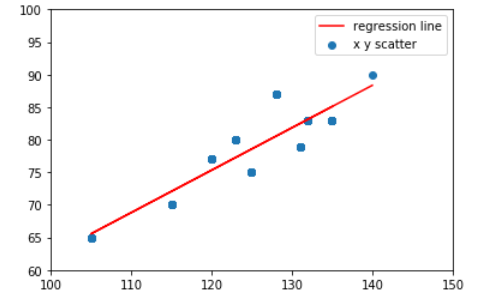
scipy.stats.linregress Model 시각화
1
2
3
4
5
6
7
#결과 시각화하여 살펴보기
plt.scatter(x, y)
plt.xlim([100,150])
plt.ylim([60,100])
plt.plot(x,0.6514309527270075*x-2.8564471221974657,'r')
plt.legend(["regression line", "x y scatter"])
plt.show()
scipy.stats.linregress 을 활용하여 모집단과 표본집단을 사용할 경우로 나누었다.
모집단: 전체 대상 또는 전체 집합
표본집단: 모집단의 부분집합
모집단에서 표본집단을 추출하는 방법은 다음과 같이 4개가 있다.
- 단순임의추출: 임의로 추출
- 계통추출: 표본 원소에 번호를 부여한 후 표본의 크기 K값 정함 => 난수표를 이용하여 K-1의 숫자중 하나를 선택하고 그 숫자에 K만큼 더해가며 개체를 선택
- 층화추출: 그룹의 차이가 존재하는 그룹으로 나눈뒤 그룹에서 선택
- 군집추출: 그룹간의 차이가 없는 그룹으로 나눈뒤 그룹에서 선택
모집단 이용하기
1
2
3
4
5
6
7
8
9
10
11
12
13
14
15
16
17
#모집단 자료(전체) 이용하기
print("\n <모집단 자료 이용하기>")
product = pd.read_csv("https://raw.githubusercontent.com/wjddyd66/R/master/Data/product.csv")
print(product.head(2))
print(product.corr())
model2 = stats.linregress(product["b"], product["c"])

print("model: ", model2)
print("기울기: ", model2.slope)
print("절편: ", model2.intercept)
print("상관계수: ", model2.rvalue)
print("p값: ", model2.pvalue)
print("표준오차: ", model2.stderr)
'''
상관계수:  0.766852699640837 => 매우 높은 양의 상관관계를 가지고 있다.
p값:  0.235344857549548e-52 < 0.05 => 통계적으로 유의하다.
'''
 <모집단 자료 이용하기>
   a  b  c
0  3  4  3
1  3  3  2
          a         b         c
a  1.000000  0.499209  0.467145
b  0.499209  1.000000  0.766853
c  0.467145  0.766853  1.000000
model:  LinregressResult(slope=0.7392761785971821, intercept=0.7788583344701907, rvalue=0.766852699640837, pvalue=2.235344857549548e-52, stderr=0.03822605528717565)
기울기:  0.7392761785971821
절편:  0.7788583344701907
상관계수:  0.766852699640837
p값:  2.235344857549548e-52
표준오차:  0.03822605528717565
'\n상관계수:  0.766852699640837 => 매우 높은 양의 상관관계를 가지고 있다.\np값:  0.235344857549548e-52 < 0.05 => 통계적으로 유의하다.\n'
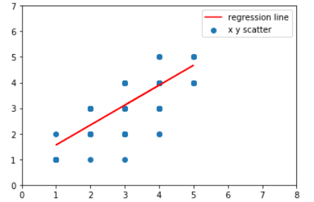
모집단 Model 시각화
1
2
3
4
5
6
7
#결과 시각화하여 살펴보기
plt.scatter(product["b"], product["c"])
plt.xlim([0,8])
plt.ylim([0,7])
plt.plot(product["b"],0.7788583344701907*product["b"]+0.7788583344701907,'r')
plt.legend(["regression line", "x y scatter"])
plt.show()
표본집단(단순임의 추출) 이용하기
1
2
3
4
5
6
7
8
9
10
11
12
13
14
15
16
17
#샘플링 자료 이용하기
print("\n <샘플링 자료 이용하기>")
idx = np.random.randint(1, len(product), 150)
print(len(idx))
dataset = product.loc[idx]
print(dataset[:5])
model3 = stats.linregress(dataset["b"], dataset["c"])
print("model: ", model3)
print("기울기: ", model3.slope)
print("절편: ", model3.intercept)
print("상관계수: ", model3.rvalue)
print("p값: ", model3.pvalue)
print("표준오차: ", model3.stderr)
'''
상관계수:  0.7953597521219435 => 매우 높은 양의 상관관계를 가지고 있다.
p값:  5.424928391628453e-34 < 0.05 => 통계적으로 유의하다.
'''
 <샘플링 자료 이용하기>
150
     a  b  c
77   1  1  1
148  3  3  3
234  3  3  3
159  3  4  4
172  2  2  3
model:  LinregressResult(slope=0.7257880124122156, intercept=0.7924220153519537, rvalue=0.7953597521219435, pvalue=5.424928391628453e-34, stderr=0.045465983691246346)
기울기:  0.7257880124122156
절편:  0.7924220153519537
상관계수:  0.7953597521219435
p값:  5.424928391628453e-34
표준오차:  0.045465983691246346
'\n상관계수:  0.7953597521219435 => 매우 높은 양의 상관관계를 가지고 있다.\np값:  5.424928391628453e-34 < 0.05 => 통계적으로 유의하다.\n'
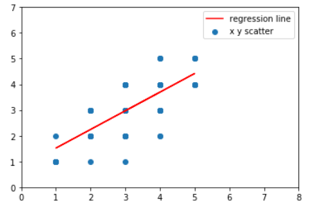
표본집단(단순임의 추출) Model 시각화
1
2
3
4
5
6
7
#결과 시각화하여 살펴보기
plt.scatter(product["b"], product["c"])
plt.xlim([0,8])
plt.ylim([0,7])
plt.plot(product["b"],0.7257880124122156*product["b"]+0.7924220153519537,'r')
plt.legend(["regression line", "x y scatter"])
plt.show()
참조: 원본코드
코드에 문제가 있거나 궁금한 점이 있으면 wjddyd66@naver.com으로 Mail을 남겨주세요.
Leave a comment