Appendix1.Numpy

Appendix1. Numpy

Numpy에서 Tool사용방법을 알아봤으나, 기초적인 부분에 대해서만 알아보고 많이 부족하다는 것을 깨달았다.
따라서 이번 Post는 Hands-on ML에서 부록 중 하나인 Numpy사용법을 알아보는 Post이다.
Tensorflow나 Pytorch에서도 기본적으로 다루는 자료형 이고, 꼭 필요한 Tool이다.
코드참조:Handson-ml2 Github

필요한 Library import

%matplotlib inline
import matplotlib.pyplot as plt
import numpy as np
import os

Creating arrays

np.zeros
모든 행렬의 값을 0으로서 채워넣는다. Input으로 Array의 Size를 지정하게 된다.

Some Vocabulary
몇몇 지정된 단어가 존재한다.

• axis: 각각의 Dimension
• rank: number of axes
• shape: list of axis length
• size: total number of elements

ex) 3x4 matrix

• rank:2
• first axis: 3 length
• second axis: 4 lenght
• shape: (3,4)
• size: 12(3*4)

Array type
Numpy Array는 ndarray type이다.

np.ones
지정한 Shape대로 모든 elements를 1로서 채운다.

np.full
지정한 Shape대로 모든 elements를 지정한 숫자로 채운다.

np.empty
지정한 Shape대로 모든 elements를 채우지 않는다.(이것은 Memery에 있는 내용이므로 예측할 수 없다.)

np.array
특정한 수를 대입하는 것이 아닌 지정한 숫자를 입력하여 Numpy Array를 구성할 수 있다.

np.arrange
Start ~ End구간을 특정한 Intervel만큼 차이나게 값을 대입할 수 있다.

np.linspace
Start ~ End구간을 특정한 개수로 나눌 수 있다.(각각의 Elements들의 Intervel은 동일)

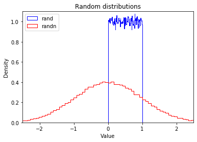
np.rand, np.randn

• np.rand: 균일 분포로서 Random하게 Sampling(0~1)
• np.randn: Gaussian 분포로서 Random하게 Sampling

np.fromfunction
사용자가 지정한 Function으로 Numpy Array의 값을 지정할 수 있다.

print('np.zeros')
print('1 Dimension')
print(np.zeros(5))
print()
print('2 Dimension')
print(np.zeros((3,4)))
print()
print('N Dimension')
print(np.zeros((2,3,4)))
print()

print('Some Vocabulary')
a = np.zeros((3,4))
print('(3,4) Matrix shape: ',a.shape)
print('(3,4) Matrix Ndim: ',a.ndim)
print('(3,4) Matrix size: ',a.size)
print()

print('Array type')
print(type(a))
print()

print('np.ones')
print(np.ones((3,4)))
print()

print('np.full')
print(np.full((3,4),np.pi))
print()

print('np.empty')
print(np.empty([2,3],dtype=float))
print()

print('np.array')
print(np.array([[1,2,3,4],[10,20,30,40]]))
print()

print('np.arange')
print('Default')
print(np.arange(1,5))
print('Specific Intervel')
print(np.arange(1,5,0.5))
print()

print('np.linspace')
print(np.linspace(0,5/3,6))
print()

print('np.rand, np.randn')
plt.hist(np.random.rand(100000), density=True, bins=100, histtype="step", color="blue", label="rand")
plt.hist(np.random.randn(100000), density=True, bins=100, histtype="step", color="red", label="randn")
plt.axis([-2.5, 2.5, 0, 1.1])
plt.legend(loc = "upper left")
plt.title("Random distributions")
plt.xlabel("Value")
plt.ylabel("Density")
plt.show()

print('np.fromfunction')
def my_function(z,y,x):
    return x*y+z

print(np.fromfunction(my_function,(3,2,10)))

np.zeros
1 Dimension
[0. 0. 0. 0. 0.]

2 Dimension
[[0. 0. 0. 0.]
 [0. 0. 0. 0.]
 [0. 0. 0. 0.]]

N Dimension
[[[0. 0. 0. 0.]
  [0. 0. 0. 0.]
  [0. 0. 0. 0.]]

 [[0. 0. 0. 0.]
  [0. 0. 0. 0.]
  [0. 0. 0. 0.]]]

Some Vocabulary
(3,4) Matrix shape:  (3, 4)
(3,4) Matrix Ndim:  2
(3,4) Matrix size:  12

Array type
<class 'numpy.ndarray'>

np.ones
[[1. 1. 1. 1.]
 [1. 1. 1. 1.]
 [1. 1. 1. 1.]]

np.full
[[3.14159265 3.14159265 3.14159265 3.14159265]
 [3.14159265 3.14159265 3.14159265 3.14159265]
 [3.14159265 3.14159265 3.14159265 3.14159265]]

np.empty
[[0. 0. 0.]
 [0. 0. 0.]]

np.array
[[ 1  2  3  4]
 [10 20 30 40]]

np.arange
Default
[1 2 3 4]
Specific Intervel
[1.  1.5 2.  2.5 3.  3.5 4.  4.5]

np.linspace
[0.         0.33333333 0.66666667 1.         1.33333333 1.66666667]

np.rand, np.randn

np.fromfunction
[[[ 0.  0.  0.  0.  0.  0.  0.  0.  0.  0.]
  [ 0.  1.  2.  3.  4.  5.  6.  7.  8.  9.]]

 [[ 1.  1.  1.  1.  1.  1.  1.  1.  1.  1.]
  [ 1.  2.  3.  4.  5.  6.  7.  8.  9. 10.]]

 [[ 2.  2.  2.  2.  2.  2.  2.  2.  2.  2.]
  [ 2.  3.  4.  5.  6.  7.  8.  9. 10. 11.]]]

Array data

dtype
Numpy는 Tensor와 마찬가지로 하나의 ndarray안의 Elements끼리는 dtype이 동일하다.
Numpy가 지원하는 Dtype은 Documnetation을 참조하자.

itemsize
Ndarray의 Elements의 Size(bytes)를 나타낸다.

print('{0:<30} {1:<10} {2:<10}'.format('Numpy','dtype','itemsize'))
a = np.arange(1,5)
b = np.arange(1.0,5.0)
c = np.arange(1,5,dtype=np.complex64)

print('{0:<30} {1:<10} {2:<10}'.format(str(a),str(a.dtype),str(a.itemsize)))
print('{0:<30} {1:<10} {2:<10}'.format(str(b),str(b.dtype),str(b.itemsize)))
print('{0:<30} {1:<10} {2:<10}'.format(str(c),str(c.dtype),str(c.itemsize)))

Numpy                          dtype      itemsize  
[1 2 3 4]                      int32      4         
[1. 2. 3. 4.]                  float64    8         
[1.+0.j 2.+0.j 3.+0.j 4.+0.j]  complex64  8         

Reshaping an array

In place
Numpy Array는 shape를 변형하는 것은 가능하지만, size는 반드시 동일하여야 한다.

reshape
reshape를 사용하여 shape를 변형하게 되면 같은 데이터를 가진 data를 Return한다. 중요한 것은 Return한 object의 값을 변형하면 이전의 data또한 값이 변형된다는 것 이다.(Shape는 달라도 변형된다.)

ravel
Numpy Array를 Flatten한 1 Dimension으로 변형시킨다.

print('In place')
print('Original')
g = np.arange(24)
print(g)
print("Rank:", g.ndim)
print()
print('Change (1,24) -> (6,4)')
g.shape = (6, 4)
print(g)
print("Rank:", g.ndim)
print()
print('Change (6,4) -> (2,3,4)')
g.shape = (2, 3, 4)
print(g)
print("Rank:", g.ndim)
print()


print('reshape')
g2 = g.reshape(4,6)
print(g2)
print("Rank:", g2.ndim)
print()
print('g2[1,2] = 999 -> g[0,2,0] = 999')
g2[1, 2] = 999
print('g')
print(g)
print('g2')
print(g2)
print()

print('ravel')
print(g.ravel())

In place
Original
[ 0  1  2  3  4  5  6  7  8  9 10 11 12 13 14 15 16 17 18 19 20 21 22 23]
Rank: 1

Change (1,24) -> (6,4)
[[ 0  1  2  3]
 [ 4  5  6  7]
 [ 8  9 10 11]
 [12 13 14 15]
 [16 17 18 19]
 [20 21 22 23]]
Rank: 2

Change (6,4) -> (2,3,4)
[[[ 0  1  2  3]
  [ 4  5  6  7]
  [ 8  9 10 11]]

 [[12 13 14 15]
  [16 17 18 19]
  [20 21 22 23]]]
Rank: 3

reshape
[[ 0  1  2  3  4  5]
 [ 6  7  8  9 10 11]
 [12 13 14 15 16 17]
 [18 19 20 21 22 23]]
Rank: 2

g2[1,2] = 999 -> g[0,2,0] = 999
g
[[[  0   1   2   3]
  [  4   5   6   7]
  [999   9  10  11]]

 [[ 12  13  14  15]
  [ 16  17  18  19]
  [ 20  21  22  23]]]
g2
[[  0   1   2   3   4   5]
 [  6   7 999   9  10  11]
 [ 12  13  14  15  16  17]
 [ 18  19  20  21  22  23]]

ravel
[  0   1   2   3   4   5   6   7 999   9  10  11  12  13  14  15  16  17
  18  19  20  21  22  23]

Arothmetic operations

기본적인 산수 연산(+, -, *, /, //, **, etc.)이 사용 가능하다.
조심하여야 하는 것은 Matrix operation이 아니라 Numpy Elements각각의 operations라는 것을 명심하여야 한다.

a = np.array([14, 23, 32, 41])
b = np.array([5,  4,  3,  2])
print('a: ',a)
print('b: ',b)
print("a + b  =", a + b)
print("a - b  =", a - b)
print("a * b  =", a * b)
print("a / b  =", a / b)
print("a // b  =", a // b)
print("a % b  =", a % b)
print("a ** b =", a ** b)

a:  [14 23 32 41]
b:  [5 4 3 2]
a + b  = [19 27 35 43]
a - b  = [ 9 19 29 39]
a * b  = [70 92 96 82]
a / b  = [ 2.8         5.75       10.66666667 20.5       ]
a // b  = [ 2  5 10 20]
a % b  = [4 3 2 1]
a ** b = [537824 279841  32768   1681]

Broadcasting

Numpy는 기본적으로 same shape가 아니면 계산되지 않으나, Broadcasting되는 몇몇 룰이 존재한다.

First rule
만약 행렬의 rank가 맞지 않는다면 계속하여 앞에 1씩 Dimension을 더해가면서 Broadcasting을 실시하게 된다.

h = np.arange(5).reshape(1, 1, 5)
print(h)
print(h + [10, 20, 30, 40, 50])  # same as: h + [[[10, 20, 30, 40, 50]]]

[[[0 1 2 3 4]]]
[[[10 21 32 43 54]]]

Second rule
만약 Dimension 중 1이있는 Array는 자동적으로 큰 Dimension(같은 값)으로서 Broadcasting된다.

k = np.arange(6).reshape(2, 3)
print(k)
print(k + [[100], [200]])  # same as: k + [[100, 100, 100], [200, 200, 200]]

[[0 1 2]
 [3 4 5]]
[[100 101 102]
 [203 204 205]]

first rule + second rule

print(k + [100, 200, 300])  # after rule 1: [[100, 200, 300]], and after rule 2: [[100, 200, 300], [100, 200, 300]]

print(k + 1000)  # same as: k + [[1000, 1000, 1000], [1000, 1000, 1000]]

[[100 201 302]
 [103 204 305]]
[[1000 1001 1002]
 [1003 1004 1005]]

Upcasting
위에서 Numpy Array는 동일한 dtype을 가진다고 하였다.
이러한 dtype은 upcasting가능하다.

k1 = np.arange(0, 5, dtype=np.uint8)
print(k1.dtype, k1)

k2 = k1 + np.array([5, 6, 7, 8, 9], dtype=np.int8)
print(k2.dtype, k2)

k3 = k1 + 1.5
print(k3.dtype, k3)

uint8 [0 1 2 3 4]
int16 [ 5  7  9 11 13]
float64 [1.5 2.5 3.5 4.5 5.5]

Conditional operators

Conditional operators는 각각의 elements or broadcasting혹인 indexing에서도 사용 가능하다.

m = np.array([20, -5, 30, 40])
print(m < [15, 16, 35, 36])

# bradcasting
print(m<25)

# indexing
print(m[m<25])

[False  True  True False]
[ True  True False False]
[20 -5]

Mathematical and statstical functions

많은 function들이 이미 ndarray에서 바로 사용 가능하다.

a = np.array([[-2.5, 3.1, 7], [10, 11, 12]])

for func in (a.min, a.max, a.sum, a.prod, a.std, a.var):
    print(func.__name__, "=", func())

min = -2.5
max = 12.0
sum = 40.6
prod = -71610.0
std = 5.084835843520964
var = 25.855555555555554

특히 많이 사용되는 것은 .sum()으로서 Numpy Array안에서 Elements끼리의 합을 구하는 것 이다.
이러한 것 중 중요한 것은 axis를 활용하여 합치는 기준 축을 잘 지정하는 것 이다.

c=np.arange(24).reshape(2,3,4)
print(c)
print('c.sum(axis=0)')
print(c.sum(axis=0))  # sum across matrices
print()

print('c.sum(axis=1)')
print(c.sum(axis=1))  # sum across row
print()

print('c.sum(axis=2)')
print(c.sum(axis=2))  # sum across columns
print()

[[[ 0  1  2  3]
  [ 4  5  6  7]
  [ 8  9 10 11]]

 [[12 13 14 15]
  [16 17 18 19]
  [20 21 22 23]]]
c.sum(axis=0)
[[12 14 16 18]
 [20 22 24 26]
 [28 30 32 34]]

c.sum(axis=1)
[[12 15 18 21]
 [48 51 54 57]]

c.sum(axis=2)
[[ 6 22 38]
 [54 70 86]]

​

Universal functions
보편적인 기능을 가진 ufunc라고 불리는 기능이 존재한다.
각각의 Elements에 적용할 수 있는 Function들이다.

a = np.array([[-2.5, 3.1, 7], [10, 11, 12]])
print("Original ndarray")
print(a)
for func in (np.square, np.abs, np.sqrt, np.exp, np.log, np.sign, np.ceil, np.modf, np.isnan, np.cos):
    print("\n", func.__name__)
    print(func(a))

Original ndarray
[[-2.5  3.1  7. ]
 [10.  11.  12. ]]

 square
[[  6.25   9.61  49.  ]
 [100.   121.   144.  ]]

 absolute
[[ 2.5  3.1  7. ]
 [10.  11.  12. ]]

 sqrt
[[       nan 1.76068169 2.64575131]
 [3.16227766 3.31662479 3.46410162]]

 exp
[[8.20849986e-02 2.21979513e+01 1.09663316e+03]
 [2.20264658e+04 5.98741417e+04 1.62754791e+05]]

 log
[[       nan 1.13140211 1.94591015]
 [2.30258509 2.39789527 2.48490665]]

 sign
[[-1.  1.  1.]
 [ 1.  1.  1.]]

 ceil
[[-2.  4.  7.]
 [10. 11. 12.]]

 modf
(array([[-0.5,  0.1,  0. ],
       [ 0. ,  0. ,  0. ]]), array([[-2.,  3.,  7.],
       [10., 11., 12.]]))

 isnan
[[False False False]
 [False False False]]

 cos
[[-0.80114362 -0.99913515  0.75390225]
 [-0.83907153  0.0044257   0.84385396]]

​

Binary ufuncs
두개의 Numpy Array의 값을 비교하거나 다른 기능의 Function을 적용할 수 있다.

a = np.array([1, -2, 3, 4])
b = np.array([2, 8, -1, 7])
print(np.add(a, b))  # equivalent to a + b
print(np.greater(a, b))  # equivalent to a > b

[ 3  6  2 11]
[False False  True False]

Array indexing

One-dimensional arrays
One-dimensional Numpy는 Python의 Array와 동일하게 Indexing이 가능하다.

a = np.array([1, 5, 3, 19, 13, 7, 3])
print('a: ',a)
# Point
print(a[3])
# Range
print(a[2:5])
print(a[2:-1])
# Reverse
print(a[::-1])
# [Start_index:End_index:Intervel]
print(a[2::2])

a:  [ 1  5  3 19 13  7  3]
19
[ 3 19 13]
[ 3 19 13  7]
[ 3  7 13 19  3  5  1]
[ 3 13  3]

Differences with regular python arrays
Numpy Array는 Broadcasting을 진행하기 때문에 Range에 값을 대입하여도 알아서 값이 잘 바뀐다.

a[2:5] = -1
print(a)

[ 1  5 -1 -1 -1  7  3]

배열이 Size가 맞지 않는 값은 대입할 수 없으며, Elements를 del을 사용하여 없앨 수 없다.

try:
    a[2:5] = [1,2,3,4,5,6]  # too long
except ValueError as e:
    print(e)
    
try:
    del a[2:5]
except ValueError as e:
    print(e)

cannot copy sequence with size 6 to array axis with dimension 3
cannot delete array elements

Numpy Array의 Slice하여 사용하는 것은 실제 Data를 복사하여 가져오는 것이 아니라 참조하여 볼 곳을 정하는 것이다.(views on the same data buffer) 이러한 특성 때문에 Slice한 값을 변경하면 Original도 변경이 되고, Original의 값을 바꾸면 Slice한 값에 영향을 미친다.
이러한 참조방식이 싫으면 .copy()를 활용하여 Data의 값을 다른 Buffer에 옮겨와서 사용하는 수 밖에 없다.

a_slice = a[2:6]
a_slice[1] = 1000
print(a)  # the original array was modified!

a[3] = 2000
print(a_slice)  # similarly, modifying the original array modifies the slice!

another_slice = a[2:6].copy()
another_slice[1] = 3000
print(a)  # the original array is untouched

a[3] = 4000
print(another_slice)  # similary, modifying the original array does not affect the slice copy

[   1    5   -1 1000   -1    7    3]
[  -1 2000   -1    7]
[   1    5   -1 2000   -1    7    3]
[  -1 3000   -1    7]

Multi-diensional arrays
다양한 차원의 Array또한 Indexing하는 것은 One-diensional arrays와 비슷하다.

b = np.arange(48).reshape(4, 12)
print(b)
print()

print(b[1, 2])  # row 1, col 2
print(b[1, :])  # row 1, all columns
print(b[:, 1])  # all rows, column 1
print()

print('Caution')
print(b[1, :]) # 1D Array of shape(12,)
print(b[1:2, :]) # 2D Array of shape(1,12)

[[ 0  1  2  3  4  5  6  7  8  9 10 11]
 [12 13 14 15 16 17 18 19 20 21 22 23]
 [24 25 26 27 28 29 30 31 32 33 34 35]
 [36 37 38 39 40 41 42 43 44 45 46 47]]

14
[12 13 14 15 16 17 18 19 20 21 22 23]
[ 1 13 25 37]

Caution
[12 13 14 15 16 17 18 19 20 21 22 23]
[[12 13 14 15 16 17 18 19 20 21 22 23]]

Fancy indexing
Range로서 값을 지정할 수도 있고, (a,b,…)처럼 Discrete한 값으로서 Indexing의 Argument로서 대입 가능하다.

print(b[(0,2), 2:5]) # rows 0 and 2, columns 2 to 4 (5-1)
print()
print(b[:, (-1, 2, -1)]) # all rows, columns -1 (last), 2 and -1 (again, and in this order)

[[ 2  3  4]
 [26 27 28]]

[[11  2 11]
 [23 14 23]
 [35 26 35]
 [47 38 47]]

Ellipsis(…)
ellipsis(…)는 특정하지 않고 모든 axes를 선택하는 경우 사용 된다.

c = b.reshape(4,2,6)
print('c')
print(c)

print(c[2, ...])  #  matrix 2, all rows, all columns.  This is equivalent to c[2, :, :]
print(c[2, 1, ...])  # matrix 2, row 1, all columns.  This is equivalent to c[2, 1, :]
print(c[2, ..., 3])  # matrix 2, all rows, column 3.  This is equivalent to c[2, :, 3]

c
[[[ 0  1  2  3  4  5]
  [ 6  7  8  9 10 11]]

 [[12 13 14 15 16 17]
  [18 19 20 21 22 23]]

 [[24 25 26 27 28 29]
  [30 31 32 33 34 35]]

 [[36 37 38 39 40 41]
  [42 43 44 45 46 47]]]
[[24 25 26 27 28 29]
 [30 31 32 33 34 35]]
[30 31 32 33 34 35]
[27 33]

Boolean indexing
Indexing에서 많이 쓰이는 방법 중 하나이다.
원하는 Column or Row의 값을 True or False로서 지정하여 Indexing을 실시한다.

b = np.arange(48).reshape(4, 12)
print(b)
print()

rows_on = np.array([True, False, True, False])
print(b[rows_on, :])  # Rows 0 and 2, all columns. Equivalent to b[(0, 2), :]
print()

cols_on = np.array([False, True, False] * 4)
print(b[:, cols_on])  # All rows, columns 1, 4, 7 and 10

[[ 0  1  2  3  4  5  6  7  8  9 10 11]
 [12 13 14 15 16 17 18 19 20 21 22 23]
 [24 25 26 27 28 29 30 31 32 33 34 35]
 [36 37 38 39 40 41 42 43 44 45 46 47]]

[[ 0  1  2  3  4  5  6  7  8  9 10 11]
 [24 25 26 27 28 29 30 31 32 33 34 35]]

[[ 1  4  7 10]
 [13 16 19 22]
 [25 28 31 34]
 [37 40 43 46]]

Iterating

Iterating또한 Python의 방식과 매우 유사하다.
기준은 Numpy Array의 First axis이다.

c = np.arange(24).reshape(2, 3, 4)  # A 3D array (composed of two 3x4 matrices)
print(c)
print()

# Standard is First axis of Numpy Array
for m in c:
    print("Item:")
    print(m)
    
# if you want see all elements -> You can use .flat
for i in c.flat:
    print("Item:", i)

[[[ 0  1  2  3]
  [ 4  5  6  7]
  [ 8  9 10 11]]

 [[12 13 14 15]
  [16 17 18 19]
  [20 21 22 23]]]

Item:
[[ 0  1  2  3]
 [ 4  5  6  7]
 [ 8  9 10 11]]
Item:
[[12 13 14 15]
 [16 17 18 19]
 [20 21 22 23]]
Item: 0
Item: 1
Item: 2
Item: 3
Item: 4
Item: 5
Item: 6
Item: 7
Item: 8
Item: 9
Item: 10
Item: 11
Item: 12
Item: 13
Item: 14
Item: 15
Item: 16
Item: 17
Item: 18
Item: 19
Item: 20
Item: 21
Item: 22
Item: 23

Stacking arrays

Numpy Array를 합치는 방법이다.

vstack
Numpy Array를 세로로 합친다.

hstack
Numpy Array를 가로로 합친다.

concatenate
axis를 기준으로 vsatck, hstack이 가능하다.

stack
새로운 Dimension을 추가하여 Numpy Array를 합친다.

q1 = np.full((3,4), 1.0)
q2 = np.full((4,4), 2.0)
q3 = np.full((3,4), 3.0)

print('q1')
print(q1)
print('q2')
print(q2)
print('q3')
print(q3)
print()

print('vstack(q1,q2,q3)')
q4 = np.vstack((q1,q2,q3))
print(q4)
print(q4.shape)
print()

print('hstack(q1,q3)')
q5 = np.hstack((q1,q3))
print(q5)
print(q5.shape)
print()

print('If Dimension is different each other')
try:
    q5 = np.hstack((q1,q2,q3))
except ValueError as e:
    print(e)
    print()
    
print('concatenate')
q7 = np.concatenate((q1,q2,q3),axis=0)
print(q7)
print(q7.shape)
print()

print('stack')
q8 = np.stack((q1,q3))
print(q8)
print(q8.shape)

q1
[[1. 1. 1. 1.]
 [1. 1. 1. 1.]
 [1. 1. 1. 1.]]
q2
[[2. 2. 2. 2.]
 [2. 2. 2. 2.]
 [2. 2. 2. 2.]
 [2. 2. 2. 2.]]
q3
[[3. 3. 3. 3.]
 [3. 3. 3. 3.]
 [3. 3. 3. 3.]]

vstack(q1,q2,q3)
[[1. 1. 1. 1.]
 [1. 1. 1. 1.]
 [1. 1. 1. 1.]
 [2. 2. 2. 2.]
 [2. 2. 2. 2.]
 [2. 2. 2. 2.]
 [2. 2. 2. 2.]
 [3. 3. 3. 3.]
 [3. 3. 3. 3.]
 [3. 3. 3. 3.]]
(10, 4)

hstack(q1,q3)
[[1. 1. 1. 1. 3. 3. 3. 3.]
 [1. 1. 1. 1. 3. 3. 3. 3.]
 [1. 1. 1. 1. 3. 3. 3. 3.]]
(3, 8)

If Dimension is different each other
all the input array dimensions for the concatenation axis must match exactly, but along dimension 0, the array at index 0 has size 3 and the array at index 1 has size 4

concatenate
[[1. 1. 1. 1.]
 [1. 1. 1. 1.]
 [1. 1. 1. 1.]
 [2. 2. 2. 2.]
 [2. 2. 2. 2.]
 [2. 2. 2. 2.]
 [2. 2. 2. 2.]
 [3. 3. 3. 3.]
 [3. 3. 3. 3.]
 [3. 3. 3. 3.]]
(10, 4)

stack
[[[1. 1. 1. 1.]
  [1. 1. 1. 1.]
  [1. 1. 1. 1.]]

 [[3. 3. 3. 3.]
  [3. 3. 3. 3.]
  [3. 3. 3. 3.]]]
(2, 3, 4)

Splitting arrays

위의 Stacking과 다르게 array를 splitting하는 방법 또한 존재한다. Stacking과 연관지어 vstack -> vsplit, hstack -> hsplit으로 변형시키면 된다.

r = np.arange(24).reshape(6,4)
print('Original')
print(r)
print()

print('Vsplit')
v1,v2,v3 = np.vsplit(r,3)
print('v1')
print(v1)
print('v2')
print(v2)
print('v3')
print(v3)
print()

print('Hsplit')
h1,h2 = np.hsplit(r,2)
print('h1')
print(h1)
print('h2')
print(h2)
print()

print('Split with axis option')
s1,s2 = np.split(r,2,axis=1)
print('s1')
print(s1)
print('s2')
print(s2)

Original
[[ 0  1  2  3]
 [ 4  5  6  7]
 [ 8  9 10 11]
 [12 13 14 15]
 [16 17 18 19]
 [20 21 22 23]]

Vsplit
v1
[[0 1 2 3]
 [4 5 6 7]]
v2
[[ 8  9 10 11]
 [12 13 14 15]]
v3
[[16 17 18 19]
 [20 21 22 23]]

Hsplit
h1
[[ 0  1]
 [ 4  5]
 [ 8  9]
 [12 13]
 [16 17]
 [20 21]]
h2
[[ 2  3]
 [ 6  7]
 [10 11]
 [14 15]
 [18 19]
 [22 23]]

Split with axis option
s1
[[ 0  1]
 [ 4  5]
 [ 8  9]
 [12 13]
 [16 17]
 [20 21]]
s2
[[ 2  3]
 [ 6  7]
 [10 11]
 [14 15]
 [18 19]
 [22 23]]

Saving and loading

Binary .npy format
Numpy는 np.save()로서 저장하고 np.load()로서 저장한 Numpy Array를 불러올 수 있다.
File의 Format은 .npy이다.

print('Saving')
a = np.random.rand(2,3)
print(a)
np.save('my_array',a)
print()

print('Loading')
a_loaded = np.load('my_array.npy')
print(a_loaded)

Saving
[[0.35427376 0.3352868  0.74576787]
 [0.3903175  0.68743649 0.8433208 ]]

Loading
[[0.35427376 0.3352868  0.74576787]
 [0.3903175  0.68743649 0.8433208 ]]

Text Format
Numpy Array는 .csv FileFormat으로서 저장하고 불러올 수 있다.
.csv는 Tab으로서 구분 기호로 사용한다. 구분기호는 delimiter attribute를 통하여 사용자가 직접 지정할 수 있다.

print('Saving')
np.savetxt('my_array.csv',a, delimiter=",")
print()

print('Loading')
a_loaded = np.loadtxt('my_array.csv',delimiter=',')
print(a_loaded)

Saving

Loading
[[0.35427376 0.3352868  0.74576787]
 [0.3903175  0.68743649 0.8433208 ]]

Zipped .npz format
여러개의 Numpy Array를 하나의 zipped file에 저장할 수 있다.
np.savez()로서 저장할 수 있고, 불러오는 것은 np.load()로서 동일하다.
저장 Format은 .npz이고, key:numpy형식으로 저장된다.

b = np.arange(24,dtype=np.uint8).reshape(2,3,4)
print('b')
print(b)
print()

np.savez('my_arrays',my_a=a, my_b=b)
my_arrays = np.load('my_arrays.npz')
print('my_arrays')
print(my_arrays)
print()

print('my_arrays keys')
for k in my_arrays.keys():
    print(k)
print()

print('my_b')
print(my_arrays['my_b'])
print(type(my_arrays['my_b']))

b
[[[ 0  1  2  3]
  [ 4  5  6  7]
  [ 8  9 10 11]]

 [[12 13 14 15]
  [16 17 18 19]
  [20 21 22 23]]]

my_arrays
<numpy.lib.npyio.NpzFile object at 0x0000017DD535D940>

my_arrays keys
my_a
my_b

my_b
[[[ 0  1  2  3]
  [ 4  5  6  7]
  [ 8  9 10 11]]

 [[12 13 14 15]
  [16 17 18 19]
  [20 21 22 23]]]
<class 'numpy.ndarray'>

---

참조: 원본코드
참조: Handson-ml2 Github

코드에 문제가 있거나 궁금한 점이 있으면 wjddyd66@naver.com으로 Mail을 남겨주세요.