Appendix2. Pandas
Pandas에서 Tool사용방법을 알아봤으나, 기초적인 부분에 대해서만 알아보고 많이 부족하다는 것을 깨달았다.
따라서 이번 Post는 Hands-on ML에서 부록 중 하나인 Pandas사용법을 알아보는 Post이다.
2D Dimension의 DataStructure에 사용하기 편하며, 많이 사용하는 DB와 같은 기능을 많이 지원해준다.
코드참조:Handson-ml2 Github
필요한 Library import
1
2
3
4
| %matplotlib inline
import matplotlib.pyplot as plt
import pandas as pd
import numpy as np
|
Series objects
Pandas의 DataStructure중에 하나이다. Series는 1D array로서 Row는 Label, Column은 1개 존재하는 DataStruecture이다.
1
2
| s = pd.Series([2,-1,3,5])
print(s)
|
1
2
3
4
5
| 0 2
1 -1
2 3
3 5
dtype: int64
|
Similar to a 1D ndarray
1 Dimension Numpy Array와 Pandas의 Series는 유사한 부분이 많다.
Arithmetic operations과 Conditional operations또한 가능하고 Numpy와 마찬가지로 Broadcasting이 가능하다.
1
2
3
4
5
6
7
8
9
10
11
12
13
14
15
| numpy = np.exp(s)
print('numpy')
print(numpy)
print()
print('Arithmetic operations elementwise')
print(s+[1000,2000,3000,4000])
print()
print('Broadcasting')
print(s+100)
print()
print('Conditional operations')
print(s<0)
|
1
2
3
4
5
6
7
8
9
10
11
12
13
14
15
16
17
18
19
20
21
22
23
24
25
26
27
| numpy
0 7.389056
1 0.367879
2 20.085537
3 148.413159
dtype: float64
Arithmetic operations elementwise
0 1002
1 1999
2 3003
3 4005
dtype: int64
Broadcasting
0 102
1 99
2 103
3 105
dtype: int64
Conditional operations
0 False
1 True
2 False
3 False
dtype: bool
|
Index labels
Series의 Index를 지정하지 않으면 자동으로 0~… 으로서 지정된다.
이러한 Index는 특별한 값으로 Labeling가능하고, Index or Label로서 Series에 접근할 수 있다.
1
2
3
4
5
6
7
8
9
10
11
12
13
14
15
| s2 = pd.Series([68, 83, 112, 68], index=["alice", "bob", "charles", "darwin"])
print(s2)
print()
print('Accessing by Labels')
print(s2['bob'])
print()
print('Accessing by Index')
print(s2[1])
print()
print('Indexing')
print(s2[1:3])
print()
|
1
2
3
4
5
6
7
8
9
10
11
12
13
14
15
16
| alice 68
bob 83
charles 112
darwin 68
dtype: int64
Accessing by Labels
83
Accessing by Index
83
Indexing
bob 83
charles 112
dtype: int64
|
Caution when Indexing Series
Series를 Indexing할 때 매우 주의하여야 하는 점 이다. Series는 처음 선언한 뒤 Indexing을 통해 Slicing이 가능하지만 한번 Slicing한 후에는 Indexing이 .iloc이 아닌 이상 안된다.
1
2
3
4
5
6
7
8
9
10
11
12
13
14
15
16
| surprise = pd.Series([1000, 1001, 1002, 1003])
surprise_slice = surprise.iloc[2:]
print(surprise_slice)
print()
# Indexing -> Indexing
print('Indexing -> Indexing')
try:
surprise_slice[0]
except KeyError as e:
print('Key Error',0)
print()
# Indexing -> Indexing by iloc
print("Indexing -> Indexing by iloc")
print(surprise_slice.iloc[0])
|
1
2
3
4
5
6
7
8
9
| 2 1002
3 1003
dtype: int64
Indexing -> Indexing
Key Error 0
Indexing -> Indexing by iloc
1002
|
Init form dict
Series는 Dict형태를 통하여 정의될 수 있고, Specific 한 Labels를 통하여 Indexing이 가능하다.
1
2
3
4
5
6
7
8
9
10
11
12
13
| # Define Series by Dict
weights = {"alice": 68, "bob": 83, "colin": 86, "darwin": 68}
s3 = pd.Series(weights)
print(s3)
print()
# Indexing by Labels
s4 = pd.Series(weights,index=["colin", "alice"])
print(s4)
print()
s5 = pd.Series(s3,index=["colin", "alice"])
print(s5)
|
1
2
3
4
5
6
7
8
9
10
11
12
13
| alice 68
bob 83
colin 86
darwin 68
dtype: int64
colin 86
alice 68
dtype: int64
colin 86
alice 68
dtype: int64
|
Automatic alignment
Series는 Operation발생시 같은 Label끼리는 Operation을 진행하지만, Label이 다른 경우는 Operation을 진행하지 않는다.
이러한 Matching되지 않는 Label끼리의 Operation결과는 NaN으로서 주어진다.
1
2
3
4
5
6
| print(s2.keys())
print(s3.keys())
print()
print('s2+s3')
print(s2+s3)
|
1
2
3
4
5
6
7
8
9
10
| Index(['alice', 'bob', 'charles', 'darwin'], dtype='object')
Index(['alice', 'bob', 'colin', 'darwin'], dtype='object')
s2+s3
alice 136.0
bob 166.0
charles NaN
colin NaN
darwin 136.0
dtype: float64
|
Init with a scalar
다양한 index labels에 같은 Scalar값을 선언할 수 있다.
1
2
| meaning = pd.Series(42,['life','universe','everything'])
print(meaning)
|
1
2
3
4
| life 42
universe 42
everything 42
dtype: int64
|
Series name
하나의 Series는 하나의 이름을 가질 수 있다.
1
2
| s6 = pd.Series([83,68],index=['bob','alice'],name='weights')
print(s6)
|
1
2
3
| bob 83
alice 68
Name: weights, dtype: int64
|
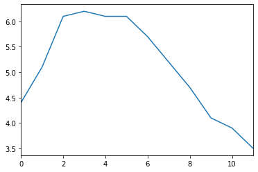
Plotting a Series
Series는 matplotlib을 통하여 간편하게 Visualization할 수 있다.
자세한 내용은 Pandas-Visualization과 Appendix3.matplotlib을 참조하자.
1
2
3
4
| temperatures = [4.4,5.1,6.1,6.2,6.1,6.1,5.7,5.2,4.7,4.1,3.9,3.5]
s7 = pd.Series(temperatures, name="Temperature")
s7.plot()
plt.show()
|
Handling time
pandas는 timestamps data를 쉽게 다룰 수 있게 되어있다.
- 2016Q3과 같은 기간이나 frequencies(such as ‘monthly’)를 다룰 수 있다.
- 기간을 시간 Data로서 변경 가능하고 그 반대또한 가능하다.
- Data를 Resampling하거나 모을 수 있다.
Time range
pd.date_range()를 통하여 Timestamps Data를 다룰 수 있다.
1
2
| dates = pd.date_range('2016/10/29 5:30pm', periods=12, freq='H')
print(dates)
|
1
2
3
4
5
6
7
| DatetimeIndex(['2016-10-29 17:30:00', '2016-10-29 18:30:00',
'2016-10-29 19:30:00', '2016-10-29 20:30:00',
'2016-10-29 21:30:00', '2016-10-29 22:30:00',
'2016-10-29 23:30:00', '2016-10-30 00:30:00',
'2016-10-30 01:30:00', '2016-10-30 02:30:00',
'2016-10-30 03:30:00', '2016-10-30 04:30:00'],
dtype='datetime64[ns]', freq='H')
|
TimeSeries는 위와 같이 Date를 Index로서 사용 가능하다.
1
2
| temp_series = pd.Series(temperatures,dates)
print(temp_series)
|
1
2
3
4
5
6
7
8
9
10
11
12
13
| 2016-10-29 17:30:00 4.4
2016-10-29 18:30:00 5.1
2016-10-29 19:30:00 6.1
2016-10-29 20:30:00 6.2
2016-10-29 21:30:00 6.1
2016-10-29 22:30:00 6.1
2016-10-29 23:30:00 5.7
2016-10-30 00:30:00 5.2
2016-10-30 01:30:00 4.7
2016-10-30 02:30:00 4.1
2016-10-30 03:30:00 3.9
2016-10-30 04:30:00 3.5
Freq: H, dtype: float64
|
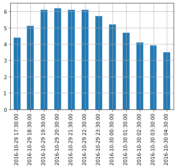
VIsualization
1
2
3
4
| temp_series.plot(kind='bar')
plt.grid(True)
plt.show()
|
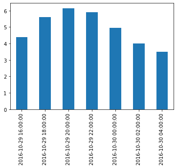
Resample
Series는 원하는 Frequency로서 ReSampling가능 하다.
아래 그림을 살펴보면 이해하기 편하다.

사진 출처:rfriends Blog
즉, 위의 Frequency가 1H인 Series를 2H로서 resampling하면 2개의 값들이 묶이게 되는 것 이다.
이렇게 묶인 값들의 .first() or .sum()과 같은 Function을 적용 가능하다.
1
2
3
4
5
6
7
| temp_series_freq_2H = temp_series.resample("2H")
print(temp_series_freq_2H)
# Apply Mean
temp_series_freq_2H = temp_series_freq_2H.mean()
temp_series_freq_2H.plot(kind="bar")
plt.show()
|
1
| DatetimeIndexResampler [freq=<2 * Hours>, axis=0, closed=left, label=left, convention=start, base=0]
|
Function을 적용하는 방법은 위와 같이 .mean()도 가능하지만 .apply(np.mean())과 같은 형식도 적용 가능하다.
1
2
| temp_series_freq_2H = temp_series.resample("2H").apply(np.mean)
print(temp_series_freq_2H)
|
1
2
3
4
5
6
7
8
| 2016-10-29 16:00:00 4.40
2016-10-29 18:00:00 5.60
2016-10-29 20:00:00 6.15
2016-10-29 22:00:00 5.90
2016-10-30 00:00:00 4.95
2016-10-30 02:00:00 4.00
2016-10-30 04:00:00 3.50
Freq: 2H, dtype: float64
|
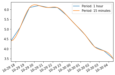
Upsampling and interpolation
위에서는 Frequency를 Decrease하였다.
Upsampling시에는 존재하지 않는 값을 NaN으로서 처리하게 되며, 이러한 NaN값을 채우는 방법은 다양하게 존재한다.
1
2
3
4
5
6
7
8
9
10
11
12
13
14
15
| print('Upsampling')
temp_series_freq_15min = temp_series.resample("15Min").mean()
print(temp_series_freq_15min.head(n=10)) # `head` displays the top n values
print()
print('Linear interpolate(cubic)')
temp_series_freq_15min = temp_series.resample("15Min").interpolate(method="cubic")
print(temp_series_freq_15min.head(n=10))
print()
# Visualization: Using interpolate is more smmother than no iterpolate
temp_series.plot(label="Period: 1 hour")
temp_series_freq_15min.plot(label="Period: 15 minutes")
plt.legend()
plt.show()
|
1
2
3
4
5
6
7
8
9
10
11
12
13
14
15
16
17
18
19
20
21
22
23
24
25
| Upsampling
2016-10-29 17:30:00 4.4
2016-10-29 17:45:00 NaN
2016-10-29 18:00:00 NaN
2016-10-29 18:15:00 NaN
2016-10-29 18:30:00 5.1
2016-10-29 18:45:00 NaN
2016-10-29 19:00:00 NaN
2016-10-29 19:15:00 NaN
2016-10-29 19:30:00 6.1
2016-10-29 19:45:00 NaN
Freq: 15T, dtype: float64
Linear interpolate(cubic)
2016-10-29 17:30:00 4.400000
2016-10-29 17:45:00 4.452911
2016-10-29 18:00:00 4.605113
2016-10-29 18:15:00 4.829758
2016-10-29 18:30:00 5.100000
2016-10-29 18:45:00 5.388992
2016-10-29 19:00:00 5.669887
2016-10-29 19:15:00 5.915839
2016-10-29 19:30:00 6.100000
2016-10-29 19:45:00 6.203621
Freq: 15T, dtype: float64
|
Timezones
각 지역마다 기준 시간이 다르다.
Pandas의 Series는 이러한 시간을 .tz_localize()를 사용하여 특정 지역에 맞게 설정할 수 있다.
1
2
3
4
5
6
7
8
| print('America/New_York')
temp_series_ny = temp_series.tz_localize("America/New_York")
print(temp_series_ny)
print()
print('Europe/Paris')
temp_series_paris = temp_series_ny.tz_convert("Europe/Paris")
print(temp_series_paris)
|
1
2
3
4
5
6
7
8
9
10
11
12
13
14
15
16
17
18
19
20
21
22
23
24
25
26
27
28
29
| America/New_York
2016-10-29 17:30:00-04:00 4.4
2016-10-29 18:30:00-04:00 5.1
2016-10-29 19:30:00-04:00 6.1
2016-10-29 20:30:00-04:00 6.2
2016-10-29 21:30:00-04:00 6.1
2016-10-29 22:30:00-04:00 6.1
2016-10-29 23:30:00-04:00 5.7
2016-10-30 00:30:00-04:00 5.2
2016-10-30 01:30:00-04:00 4.7
2016-10-30 02:30:00-04:00 4.1
2016-10-30 03:30:00-04:00 3.9
2016-10-30 04:30:00-04:00 3.5
Freq: H, dtype: float64
Europe/Paris
2016-10-29 23:30:00+02:00 4.4
2016-10-30 00:30:00+02:00 5.1
2016-10-30 01:30:00+02:00 6.1
2016-10-30 02:30:00+02:00 6.2
2016-10-30 02:30:00+01:00 6.1
2016-10-30 03:30:00+01:00 6.1
2016-10-30 04:30:00+01:00 5.7
2016-10-30 05:30:00+01:00 5.2
2016-10-30 06:30:00+01:00 4.7
2016-10-30 07:30:00+01:00 4.1
2016-10-30 08:30:00+01:00 3.9
2016-10-30 09:30:00+01:00 3.5
Freq: H, dtype: float64
|
Periods
위의 Pandas로 다룬 Data들은 시간으로서 표현되었다.
Series는 이러한 시간이 아니라 기간으로서 표현이 가능하다.
1
2
3
4
5
6
| quarters = pd.period_range('2016Q1', periods=8, freq='Q')
print(quarters)
print()
print('Arothmetic operation')
print(quarters+3)
|
1
2
3
4
5
6
7
8
| PeriodIndex(['2016Q1', '2016Q2', '2016Q3', '2016Q4', '2017Q1', '2017Q2',
'2017Q3', '2017Q4'],
dtype='period[Q-DEC]', freq='Q-DEC')
Arothmetic operation
PeriodIndex(['2016Q4', '2017Q1', '2017Q2', '2017Q3', '2017Q4', '2018Q1',
'2018Q2', '2018Q3'],
dtype='period[Q-DEC]', freq='Q-DEC')
|
Period중 좀더 Detail하게 선택하는 것은 .asfreq()를 통하여 설정할 수 있다.
1
2
3
4
5
6
| print('First of Quartile')
print(quarters.asfreq('M',how='start'))
print()
print('Last of Quartile')
print(quarters.asfreq('M'))
|
1
2
3
4
5
6
7
8
9
| First of Quartile
PeriodIndex(['2016-01', '2016-04', '2016-07', '2016-10', '2017-01', '2017-04',
'2017-07', '2017-10'],
dtype='period[M]', freq='M')
Last of Quartile
PeriodIndex(['2016-03', '2016-06', '2016-09', '2016-12', '2017-03', '2017-06',
'2017-09', '2017-12'],
dtype='period[M]', freq='M')
|
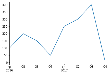
Period -> Frequency로서의 변환은 .to_timestamp로서 변경된다.
Frequency -> Period는 .to_period로서 변경된다.
1
2
3
4
5
6
7
8
9
10
11
| print('Period -> Frequency')
last_hours = quarters.to_timestamp("M")
print(last_hours)
print()
print('Frequency -> Period')
print(last_hours.to_period())
# Visualization
test = pd.Series([100,200,150,50,250,300,400,10],last_hours.to_period()).plot(kind='line')
plt.show()
|
1
2
3
4
5
6
7
8
9
| Period -> Frequency
DatetimeIndex(['2016-01-31', '2016-04-30', '2016-07-31', '2016-10-31',
'2017-01-31', '2017-04-30', '2017-07-31', '2017-10-31'],
dtype='datetime64[ns]', freq='Q-OCT')
Frequency -> Period
PeriodIndex(['2016Q1', '2016Q2', '2016Q3', '2016Q4', '2017Q1', '2017Q2',
'2017Q3', '2017Q4'],
dtype='period[Q-OCT]', freq='Q-OCT')
|
참조(Time series/ date functionality)
Time Series와 date Function에 관련된 것은 Time series/ date functionality를 참조하자.
DataFrame
DataFrame이란 Series의 집합으로 생각하면 편하다.
즉 1D Array의 집합으로서 2D Array로서 Row와 Columns로 표현하게 되고 이러한 구조는 일반적인 DB의 자료 구조와 비슷하다.
1
2
3
4
5
6
7
8
9
10
11
12
13
14
15
16
17
18
19
20
21
22
23
24
| people_dict = {
"weight": pd.Series([68, 83, 112], index=["alice", "bob", "charles"]),
"birthyear": pd.Series([1984, 1985, 1992], index=["bob", "alice", "charles"], name="year"),
"children": pd.Series([0, 3], index=["charles", "bob"]),
"hobby": pd.Series(["Biking", "Dancing"], index=["alice", "bob"]),
}
people = pd.DataFrame(people_dict)
print(people)
print()
# Access via Labels
print('Access via Labels')
print(people['birthyear'])
print()
print(people[['birthyear','hobby']])
print()
# Indexing via Specific columns & rows
d2 = pd.DataFrame(
people_dict,
columns=["birthyear", "weight", "height"],
index=["bob", "alice", "eugene"]
)
print(d2)
|
1
2
3
4
5
6
7
8
9
10
11
12
13
14
15
16
17
18
19
20
| weight birthyear children hobby
alice 68 1985 NaN Biking
bob 83 1984 3.0 Dancing
charles 112 1992 0.0 NaN
Access via Labels
alice 1985
bob 1984
charles 1992
Name: birthyear, dtype: int64
birthyear hobby
alice 1985 Biking
bob 1984 Dancing
charles 1992 NaN
birthyear weight height
bob 1984.0 83.0 NaN
alice 1985.0 68.0 NaN
eugene NaN NaN NaN
|
특정 값과 Index를 직접 지정하고 DataFrame을 지정할 수 있고, 또한 Nan값은 np.nan으로서 지정 가능하다.
1
2
3
4
5
6
7
8
9
10
11
| values = [
[1985, np.nan, "Biking", 68],
[1984, 3, "Dancing", 83],
[1992, 0, np.nan, 112]
]
d3 = pd.DataFrame(
values,
columns=["birthyear", "children", "hobby", "weight"],
index=["alice", "bob", "charles"]
)
print(d3)
|
1
2
3
4
| birthyear children hobby weight
alice 1985 NaN Biking 68
bob 1984 3.0 Dancing 83
charles 1992 0.0 NaN 112
|
위에서는 Series와 List로서 Index Data를 지정하였지만, 가장 많이 사용하는 방법으로서(개인적으로) Dict 형식으로 선언하여 자동으로 Mapping되게 할 수 있다.
1
2
3
4
5
6
7
| people = pd.DataFrame({
"birthyear": {"alice":1985, "bob": 1984, "charles": 1992},
"hobby": {"alice":"Biking", "bob": "Dancing"},
"weight": {"alice":68, "bob": 83, "charles": 112},
"children": {"bob": 3, "charles": 0}
})
print(people)
|
1
2
3
4
| birthyear hobby weight children
alice 1985 Biking 68 NaN
bob 1984 Dancing 83 3.0
charles 1992 NaN 112 0.0
|
Multi-indexing
Pandas의 모든 ROW는 같은 Columns의 수를 가지고 있다. 이러한 특징 때문에 Indexing을 할 때 Multi-Indexing이 가능하다.
아래 예시를 살펴보게 되면 public, private로서 1차적으로 Indexing하여 Dataframe을 재 구축 하였고, 2차적으로 Paris와 London으로서 나누게 되었다.
이러한 결과로서 Multi-Index중에서 Specific한 Index를 설정하고 접근하여 값을 확인할 수 있다.
1
2
3
4
5
6
7
8
9
10
11
12
13
14
15
16
17
18
19
20
| d5 = pd.DataFrame(
{
("public", "birthyear"):
{("Paris","alice"):1985, ("Paris","bob"): 1984, ("London","charles"): 1992},
("public", "hobby"):
{("Paris","alice"):"Biking", ("Paris","bob"): "Dancing"},
("private", "weight"):
{("Paris","alice"):68, ("Paris","bob"): 83, ("London","charles"): 112},
("private", "children"):
{("Paris", "alice"):np.nan, ("Paris","bob"): 3, ("London","charles"): 0}
}
)
print(d5)
print()
# Indexing via public column
print(d5['public'])
print()
# Indexing via public column & hobby column
print(d5['public','hobby'])
|
1
2
3
4
5
6
7
8
9
10
11
12
13
14
15
| public private
birthyear hobby weight children
Paris alice 1985 Biking 68 NaN
bob 1984 Dancing 83 3.0
London charles 1992 NaN 112 0.0
birthyear hobby
Paris alice 1985 Biking
bob 1984 Dancing
London charles 1992 NaN
Paris alice Biking
bob Dancing
London charles NaN
Name: (public, hobby), dtype: object
|
Dropping a level
위에서 Multi-Indexing을 통한 결과는 Level이 2단계라고 할 수 있다.
기본적인 Level -> public, private & London, Paris로서 Reconsturcting을 거쳤기 때문이다.
따라서 이러한 Level을 Down시켜 보는 방법은 columns.droplevel()로서 drop 시킬 특정 level을 Argument로 입력한다.
1
2
| d5.columns = d5.columns.droplevel(level = 0)
print(d5)
|
1
2
3
4
| birthyear hobby weight children
Paris alice 1985 Biking 68 NaN
bob 1984 Dancing 83 3.0
London charles 1992 NaN 112 0.0
|
Tranposing
T attribute를 통하여 전치 시킬 수 있다.
1
2
3
4
5
6
| Paris London
alice bob charles
birthyear 1985 1984 1992
hobby Biking Dancing NaN
weight 68 83 112
children NaN 3 0
|
Stacking and unstacking levels
stack으로서 가장 낮은 column기준으로 쌓을 수 있고, unstack으로서 풀 수 있다. unstack시 존재하지 않는 값에 대해서는 NaN으로서 처리한다.
1
2
3
4
5
6
7
8
9
10
11
12
| print('Original')
print(d6)
print()
print('Stacking')
d7 = d6.stack()
print(d7)
print()
print('Unstacking')
d8 = d7.unstack()
print(d8)
|
1
2
3
4
5
6
7
8
9
10
11
12
13
14
15
16
17
18
19
20
21
22
23
24
25
26
27
28
| Original
Paris London
alice bob charles
birthyear 1985 1984 1992
hobby Biking Dancing NaN
weight 68 83 112
children NaN 3 0
Stacking
London Paris
birthyear alice NaN 1985
bob NaN 1984
charles 1992 NaN
hobby alice NaN Biking
bob NaN Dancing
weight alice NaN 68
bob NaN 83
charles 112 NaN
children bob NaN 3
charles 0 NaN
Unstacking
London Paris
alice bob charles alice bob charles
birthyear NaN NaN 1992 1985 1984 NaN
hobby NaN NaN NaN Biking Dancing NaN
weight NaN NaN 112 68 83 NaN
children NaN NaN 0 NaN 3 NaN
|
Accessing rows
Numpy와 같이 rows를 통하여 접근이 가능하다.
.loc을 통하여 Row Label로서 접근하거나 .iloc을 통하여 Row Index로서 접근한다.
Indexing 및 Conditional Accessing, Boolean 을 사용하여 접근 모두 가능하다.
1
2
3
4
5
6
7
8
9
10
11
12
13
14
15
16
17
18
| print('Original')
print(people)
print()
print('Access via rows by using .lic')
print(people.loc['charles'])
print()
print('Access via rows by using .iloc')
print(people.iloc[2])
print()
print('Useing Boolean Array')
print(people[np.array([True, False, True])])
print()
print('Conditional Accessing')
print(people[people['birthyear']<1990])
|
1
2
3
4
5
6
7
8
9
10
11
12
13
14
15
16
17
18
19
20
21
22
23
24
25
26
27
28
29
| Original
birthyear hobby weight children
alice 1985 Biking 68 NaN
bob 1984 Dancing 83 3.0
charles 1992 NaN 112 0.0
Access via rows by using .lic
birthyear 1992
hobby NaN
weight 112
children 0
Name: charles, dtype: object
Access via rows by using .iloc
birthyear 1992
hobby NaN
weight 112
children 0
Name: charles, dtype: object
Useing Boolean Array
birthyear hobby weight children
alice 1985 Biking 68 NaN
charles 1992 NaN 112 0.0
Conditional Accessing
birthyear hobby weight children
alice 1985 Biking 68 NaN
bob 1984 Dancing 83 3.0
|
Adding and removing columns
Column을 추가하는 방법은 다음과 같다. (Row가 Mapping되지 않으면 NaN값으로 들어가게 된다.)
- Dict Type을 통하여 Row에 Mapping하여 추가
- Indexing을 통하여 순서대로 Row의 값 추가 (
.insert()사용)
- Conditional or Arthmetic operation으로서 추가
Column을 삭제하는 방법은 다음과 같다.
1
2
3
4
5
6
7
8
9
10
11
12
13
14
15
16
17
18
19
20
21
22
23
24
| print('Original')
print(people)
print()
print('Adding Columns by Conditional & Arthmetic operation')
people["age"] = 2018 - people["birthyear"] # adds a new column "age" (Arthmetic operation)
people["over 30"] = people["age"] > 30 # adds another column "over 30" (Conditional operation)
print(people)
print()
print('Removing Columns by Using .pop and del')
birthyears = people.pop("birthyear")
del people["children"]
print(people)
print()
print('Adding Columns by Using Dict')
people["pets"] = pd.Series({"bob": 0, "charles": 5, "eugene":1}) # alice is missing, eugene is ignored
print(people)
print()
print('Adding Columns by Using .insert')
people.insert(1,'height',[172,181,185])
print(people)
|
1
2
3
4
5
6
7
8
9
10
11
12
13
14
15
16
17
18
19
20
21
22
23
24
25
26
27
28
29
| Original
birthyear hobby weight children
alice 1985 Biking 68 NaN
bob 1984 Dancing 83 3.0
charles 1992 NaN 112 0.0
Adding Columns by Conditional & Arthmetic operation
birthyear hobby weight children age over 30
alice 1985 Biking 68 NaN 33 True
bob 1984 Dancing 83 3.0 34 True
charles 1992 NaN 112 0.0 26 False
Removing Columns by Using .pop and del
hobby weight age over 30
alice Biking 68 33 True
bob Dancing 83 34 True
charles NaN 112 26 False
Adding Columns by Using Dict
hobby weight age over 30 pets
alice Biking 68 33 True NaN
bob Dancing 83 34 True 0.0
charles NaN 112 26 False 5.0
Adding Columns by Using .insert
hobby height weight age over 30 pets
alice Biking 172 68 33 True NaN
bob Dancing 181 83 34 True 0.0
charles NaN 185 112 26 False 5.0
|
Assigning new columns
새롭게 columns를 추가하는 방법으로 assign()으로 추가하는 방법이 있다.
위와 같이 Arthmetic or Conditional Operation으로서 추가 가능하지만 중요한 점은 다음과 같다.
- 원래의 DataFrame은 값이 변하지 않으므로 Return Object를 선언하여 받아야 한다.
- 따라서 Assign할 시 하나하나 Assign을 하여야 추가 할 수 있다.
1
2
3
4
5
6
7
8
9
10
11
12
13
14
15
16
17
18
19
20
21
| assign_people = people.assign(
body_mass_index = people["weight"] / (people["height"] / 100) ** 2,
has_pets = people["pets"] > 0
)
print(assign_people)
print()
print('Add columns with the same time')
try:
people.assign(
body_mass_index = people["weight"] / (people["height"] / 100) ** 2,
overweight = people["body_mass_index"] > 25 # Original Data not modified -> KeyError Occur
)
except KeyError as e:
print("Key error:", e)
print()
print('Solution')
d6 = people.assign(body_mass_index = people["weight"] / (people["height"] / 100) ** 2)
print(d6.assign(overweight = d6["body_mass_index"] > 25))
|
1
2
3
4
5
6
7
8
9
10
11
12
13
14
15
16
17
18
19
20
21
22
23
| hobby height weight age over 30 pets body_mass_index \
alice Biking 172 68 33 True NaN 22.985398
bob Dancing 181 83 34 True 0.0 25.335002
charles NaN 185 112 26 False 5.0 32.724617
has_pets
alice False
bob False
charles True
Add columns with the same time
Key error: 'body_mass_index'
Solution
hobby height weight age over 30 pets body_mass_index \
alice Biking 172 68 33 True NaN 22.985398
bob Dancing 181 83 34 True 0.0 25.335002
charles NaN 185 112 26 False 5.0 32.724617
overweight
alice False
bob True
charles True
|
Evaluating an expression
Pandas의 좋은 점은 Row의 각각에 대하여 Conditional Operation에 대하여 Boolean으로서 결과를 뽑아낼 수 있다는 것 이다.
이러한 Evaluate는 evaluate로서 나타낼 수 있고 몇몇 Arrtibute를 활용하여 조건을 나타낼 수 있다.
inplace=True: .eval()시 Original DataFrame의 Column에 결과 값을 추가한다.@: Assign된 local or global 변수를 사용할 수 있다.
1
2
3
4
5
6
7
8
9
| print('Evaluating by use inplace attribution')
people.eval("body_mass_index = weight / (height/100) ** 2", inplace=True)
print(people)
print()
print('Evaluating by use @ attributes')
overweight_threshold = 30
people.eval("overweight = body_mass_index > @overweight_threshold", inplace=True)
print(people)
|
1
2
3
4
5
6
7
8
9
10
11
12
13
14
15
16
| Evaluating by use inplace attribution
hobby height weight age over 30 pets body_mass_index
alice Biking 172 68 33 True NaN 22.985398
bob Dancing 181 83 34 True 0.0 25.335002
charles NaN 185 112 26 False 5.0 32.724617
Evaluating by use @ attributes
hobby height weight age over 30 pets body_mass_index \
alice Biking 172 68 33 True NaN 22.985398
bob Dancing 181 83 34 True 0.0 25.335002
charles NaN 185 112 26 False 5.0 32.724617
overweight
alice False
bob False
charles True
|
Querting a DataFrame
DataFrame의 장점 중 하나라고 생각한다. DB와 같이 query를 통하여 특정 조건을 만족하는 Row를 검색할 수 있다.
1
| print(people.query("age > 30 and pets == 0"))
|
1
2
| hobby height weight age over 30 pets body_mass_index overweight
bob Dancing 181 83 34 True 0.0 25.335002 False
|
Sorting a DataFrame
sort_index를 사용하여 DataFrame의 Sorting가능하다.
Sorting의 기준은 Argument로 주어지는 axis에 따라 달라진다.(0=Sorting Rows, 1=Sorting Columns)
기본적으로는 Row를 기준으로 Sorting을 실시하고 Specific한 Rows를 by Attritubes를 통하여 정의할 수 있다.
또한 위와 마찬가지로 Original DataFrame에는 영향을 미치지 않으므로 inplace attributes를 통하여 영향을 줄지 안줄지 적용할 수 있다.
1
2
3
4
5
6
7
8
9
10
11
| print('Sorting Rows')
print(people.sort_index(axis=0))
print()
print('Sorting Columns')
print(people.sort_index(axis=1))
print()
print('Sorting Rows via Specific Columns & Apply to Original Data Frame')
people.sort_values(by="age", inplace=True)
print(people)
|
1
2
3
4
5
6
7
8
9
10
11
12
13
14
15
16
17
18
19
20
21
22
23
24
25
26
27
28
29
30
31
32
| Sorting Rows
hobby height weight age over 30 pets body_mass_index \
alice Biking 172 68 33 True NaN 22.985398
bob Dancing 181 83 34 True 0.0 25.335002
charles NaN 185 112 26 False 5.0 32.724617
overweight
alice False
bob False
charles True
Sorting Columns
age body_mass_index height hobby over 30 overweight pets \
alice 33 22.985398 172 Biking True False NaN
bob 34 25.335002 181 Dancing True False 0.0
charles 26 32.724617 185 NaN False True 5.0
weight
alice 68
bob 83
charles 112
Sorting Rows via Specific Columns & Apply to Original Data Frame
hobby height weight age over 30 pets body_mass_index \
charles NaN 185 112 26 False 5.0 32.724617
alice Biking 172 68 33 True NaN 22.985398
bob Dancing 181 83 34 True 0.0 25.335002
overweight
charles True
alice False
bob False
|
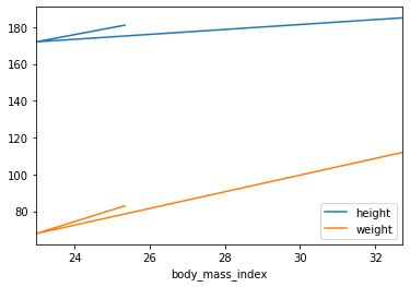
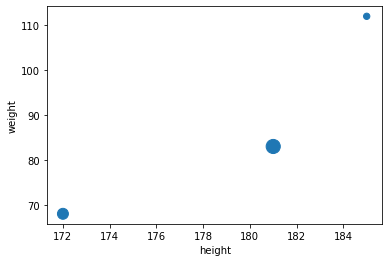
Plotting a DataFrame
Series와 같이 쉽게 .plot()을 활용하여 Visualization이 가능하다.(Visualization은 Appendix.3, 4에서 자세히 다루도록 한다.)
1
2
3
| # Visualization by Line Plot
people.plot(kind='line',x='body_mass_index',y=['height','weight'])
plt.show()
|
1
2
3
| # Visualization by Scatter plot
people.plot(kind = "scatter", x = "height", y = "weight", s=[40, 120, 200])
plt.show()
|
Operations on DataFrame
DataFrame은 Numpy와 비슷한 몇몇 Operation이 존재한다.
1
2
3
4
| # Make DataFrame
grades_array = np.array([[8,8,9],[10,9,9],[4, 8, 2], [9, 10, 10]])
grades = pd.DataFrame(grades_array, columns=["sep", "oct", "nov"], index=["alice","bob","charles","darwin"])
print(grades)
|
1
2
3
4
5
| sep oct nov
alice 8 8 9
bob 10 9 9
charles 4 8 2
darwin 9 10 10
|
- 각각의 Elements에 Operation적용 가능
- Broadcasting가능
- Arthmetic, Conditional Operation 가능
- Aggregation Operation(mean, max, sum….) 가능
all또한 Aggregation Operation이다. 각각의 Row 또는 Column에 대하여 모든 Column 또는 Row(axis로 설정)의 조건을 검사한다. <-> any
1
2
3
4
5
6
7
8
9
10
11
12
13
14
15
16
17
18
19
20
21
22
23
| print('Apply Operation to each element')
print(np.sqrt(grades))
print()
print('Broadcasting')
print(grades+1)
print()
print('Conditional Operation')
print(grades>=5)
print()
print('Aggregation Operation')
print(grades.mean())
print()
print('All Operation of Aggregation Operation(axis=0)')
print((grades>5).all())
print()
print('All Operation of Aggregation Operation(axis=1)')
print((grades>5).all(axis=1))
print()
|
1
2
3
4
5
6
7
8
9
10
11
12
13
14
15
16
17
18
19
20
21
22
23
24
25
26
27
28
29
30
31
32
33
34
35
36
37
38
39
| Apply Operation to each element
sep oct nov
alice 2.828427 2.828427 3.000000
bob 3.162278 3.000000 3.000000
charles 2.000000 2.828427 1.414214
darwin 3.000000 3.162278 3.162278
Broadcasting
sep oct nov
alice 9 9 10
bob 11 10 10
charles 5 9 3
darwin 10 11 11
Conditional Operation
sep oct nov
alice True True True
bob True True True
charles False True False
darwin True True True
Aggregation Operation
sep 7.75
oct 8.75
nov 7.50
dtype: float64
All Operation of Aggregation Operation(axis=0)
sep False
oct True
nov False
dtype: bool
All Operation of Aggregation Operation(axis=1)
alice True
bob True
charles False
darwin True
dtype: bool
|
Automatic alignment
Series와 마찬가지로 DataFrame또한 Operation을 진행할때 Index Label과 Column을 맞춰서 Operation을 진행하게 된다.
Operation 중 Argument가 하나라도 NaN이면 어떤 Operation이던간에 결과는 NaN으로 처리되고 또한, Series와 마찬가지로 일치하지 않는 Index Label이나 Column이 존재할 경우 NaN으로서 처리 된다.
1
2
3
4
5
6
7
8
9
10
11
12
| print('Grades')
print(grades.sort_index(axis=0).sort_index(axis=1))
print()
print('Bonus_points')
bonus_array = np.array([[0,np.nan,2],[np.nan,1,0],[0, 1, 0], [3, 3, 0]])
bonus_points = pd.DataFrame(bonus_array, columns=["oct", "nov", "dec"], index=["bob","colin", "darwin", "charles"])
print(bonus_points.sort_index(axis=0).sort_index(axis=1))
print()
print('After Artimetic Operation(+)')
print(grades+bonus_points)
|
1
2
3
4
5
6
7
8
9
10
11
12
13
14
15
16
17
18
19
20
21
| Grades
nov oct sep
alice 9 8 8
bob 9 9 10
charles 2 8 4
darwin 10 10 9
Bonus_points
dec nov oct
bob 2.0 NaN 0.0
charles 0.0 3.0 3.0
colin 0.0 1.0 NaN
darwin 0.0 1.0 0.0
After Artimetic Operation(+)
dec nov oct sep
alice NaN NaN NaN NaN
bob NaN NaN 9.0 NaN
charles NaN 5.0 11.0 NaN
colin NaN NaN NaN NaN
darwin NaN 11.0 10.0 NaN
|
Handling missing data
missing data란 Upsampling or Operation실시하는 경우 NaN으로서 표시되는 Data를 처리하는 방법이다.
가장 기본적인 방법으로서는 .fillna()를 통하여 NaN값을 특정값으로서 치환하거나, 사용자가 지정하는 특정값을 대입하는 방법이 존재한다.
1
2
3
4
5
6
7
8
9
10
11
| print('Use fillna Function')
print((grades + bonus_points).fillna(0))
print()
print('Assign a specific value')
fixed_bonus_points = bonus_points.fillna(0)
fixed_bonus_points.insert(0, "sep", 0)
fixed_bonus_points.loc["alice"] = 0
fixed_bonus_points = fixed_bonus_points.drop('dec',1)
fixed_bonus_points = fixed_bonus_points.drop('colin',0)
print(grades+fixed_bonus_points)
|
1
2
3
4
5
6
7
8
9
10
11
12
13
14
| Use fillna Function
dec nov oct sep
alice 0.0 0.0 0.0 0.0
bob 0.0 0.0 9.0 0.0
charles 0.0 5.0 11.0 0.0
colin 0.0 0.0 0.0 0.0
darwin 0.0 11.0 10.0 0.0
Assign a specific value
sep oct nov
alice 8 8.0 9.0
bob 10 9.0 9.0
charles 4 11.0 5.0
darwin 9 10.0 11.0
|
위와 같은 방식은 특정 값을 대입해야 하므로 분석하는데 많은 어려움을 겪을 수 있다.
따라서 Dataframe에서는 interpolate를 사용하게 되면 NaN기준으로 양옆의 값들의 평균으로 대체한다.
1
| print(bonus_points.interpolate(axis=1))
|
1
2
3
4
5
| oct nov dec
bob 0.0 1.0 2.0
colin NaN 1.0 0.0
darwin 0.0 1.0 0.0
charles 3.0 3.0 0.0
|
이와 반대로 아직 값이 정해지지 않았으나 ,Column이나 Row를 추가해야 하는 경우 np.nan으로서 NaN값을 대입할 수 있다.
1
2
3
| nan_points = bonus_points.copy()
nan_points.insert(0,'sep',np.nan)
print(nan_points)
|
1
2
3
4
5
| sep oct nov dec
bob NaN 0.0 NaN 2.0
colin NaN NaN 1.0 0.0
darwin NaN 0.0 1.0 0.0
charles NaN 3.0 3.0 0.0
|
계산 결과에서 NaN값이 나타나는 것이 싫으면 .dropna()를 활용하여 NaN값을 전부 없앨 수 있다.(axis로 기준을 정할 수 있고, how를 통하여 모든 값이 NaN이거나, 하나라도 NaN값을 포함하는 row나 Column을 없앨 수 있다.)
1
2
| drop_points = nan_points.dropna(axis=1,how='all')
print(drop_points)
|
1
2
3
4
5
| oct nov dec
bob 0.0 NaN 2.0
colin NaN 1.0 0.0
darwin 0.0 1.0 0.0
charles 3.0 3.0 0.0
|
Aggregating with groupby
SQL문과 같이 group by를 하여서 원하는 Data를 모아서 확인할 수 있다.
1
2
3
4
5
6
7
8
9
10
11
12
| # Insert new Columns
bonus_points['hobby'] = ['Biking','Dancing',np.nan,'Biking']
print(bonus_points)
print()
print('Using Group by')
grouped_grades = bonus_points.groupby('hobby')
print(grouped_grades)
print()
print('Apply Function')
print(grouped_grades.mean())
|
1
2
3
4
5
6
7
8
9
10
11
12
13
14
| oct nov dec hobby
bob 0.0 NaN 2.0 Biking
colin NaN 1.0 0.0 Dancing
darwin 0.0 1.0 0.0 NaN
charles 3.0 3.0 0.0 Biking
Using Group by
<pandas.core.groupby.generic.DataFrameGroupBy object at 0x000001407ECF3550>
Apply Function
oct nov dec
hobby
Biking 1.5 3.0 1.0
Dancing NaN 1.0 0.0
|
Pivot tables
DataFrame은 PivotTable을 지원한다.
이러한 PivotTable은 빠르게 데이터의 속성을 알 수 있으며, aggfunc를 통하여 어떠한 속성에 Focus를 맞추어서 Pivot Table을 사용할 지 정할 수 있다.
1
2
3
4
5
6
| del bonus_points['hobby']
print(bonus_points)
print()
print('Pivot Table')
print(pd.pivot_table(bonus_points,index='oct',aggfunc=np.max))
|
1
2
3
4
5
6
7
8
9
10
11
| oct nov dec
bob 0.0 NaN 2.0
colin NaN 1.0 0.0
darwin 0.0 1.0 0.0
charles 3.0 3.0 0.0
Pivot Table
dec nov
oct
0.0 2.0 1.0
3.0 0.0 3.0
|
Overview functions
DataFrame의 크기가 매우 큰 경우 몇몇 특성을 빠르게 알아보기 위하여 사용하는 Function이 존재한다.
먼저 알아보기 편하게 임의의 큰 DataFrame을 정의하자.
1
2
3
4
5
| much_data = np.fromfunction(lambda x,y: (x+y*y)%17*11, (10000, 26))
large_df = pd.DataFrame(much_data, columns=list("ABCDEFGHIJKLMNOPQRSTUVWXYZ"))
large_df[large_df % 16 == 0] = np.nan
large_df.insert(3,"some_text", "Blabla")
print(large_df)
|
1
2
3
4
5
6
7
8
9
10
11
12
13
14
15
16
17
18
19
20
21
22
23
24
25
26
27
| A B C some_text D E F G H I \
0 NaN 11.0 44.0 Blabla 99.0 NaN 88.0 22.0 165.0 143.0
1 11.0 22.0 55.0 Blabla 110.0 NaN 99.0 33.0 NaN 154.0
2 22.0 33.0 66.0 Blabla 121.0 11.0 110.0 44.0 NaN 165.0
3 33.0 44.0 77.0 Blabla 132.0 22.0 121.0 55.0 11.0 NaN
4 44.0 55.0 88.0 Blabla 143.0 33.0 132.0 66.0 22.0 NaN
... ... ... ... ... ... ... ... ... ... ...
9995 NaN NaN 33.0 Blabla 88.0 165.0 77.0 11.0 154.0 132.0
9996 NaN 11.0 44.0 Blabla 99.0 NaN 88.0 22.0 165.0 143.0
9997 11.0 22.0 55.0 Blabla 110.0 NaN 99.0 33.0 NaN 154.0
9998 22.0 33.0 66.0 Blabla 121.0 11.0 110.0 44.0 NaN 165.0
9999 33.0 44.0 77.0 Blabla 132.0 22.0 121.0 55.0 11.0 NaN
... Q R S T U V W X Y Z
0 ... 11.0 NaN 11.0 44.0 99.0 NaN 88.0 22.0 165.0 143.0
1 ... 22.0 11.0 22.0 55.0 110.0 NaN 99.0 33.0 NaN 154.0
2 ... 33.0 22.0 33.0 66.0 121.0 11.0 110.0 44.0 NaN 165.0
3 ... 44.0 33.0 44.0 77.0 132.0 22.0 121.0 55.0 11.0 NaN
4 ... 55.0 44.0 55.0 88.0 143.0 33.0 132.0 66.0 22.0 NaN
... ... ... ... ... ... ... ... ... ... ... ...
9995 ... NaN NaN NaN 33.0 88.0 165.0 77.0 11.0 154.0 132.0
9996 ... 11.0 NaN 11.0 44.0 99.0 NaN 88.0 22.0 165.0 143.0
9997 ... 22.0 11.0 22.0 55.0 110.0 NaN 99.0 33.0 NaN 154.0
9998 ... 33.0 22.0 33.0 66.0 121.0 11.0 110.0 44.0 NaN 165.0
9999 ... 44.0 33.0 44.0 77.0 132.0 22.0 121.0 55.0 11.0 NaN
[10000 rows x 27 columns]
|
head(): 상위 5개의 정보를 살필 수 있다. (Argument로서 몇개의 Row를 볼지는 정할 수 있다.)tail(): 하위 5개의 정보를 살필 수 있다. (Argument로서 몇개의 Row를 볼지는 정할 수 있다.)info(): Column의 내용을 요약하여 살필 수 있다.describe(): 주요사용하는 값들에 대하여 살펴볼 수 있다.
1
2
| print('Head')
print(large_df.head(n=3))
|
1
2
3
4
5
6
7
8
9
10
11
12
| Head
A B C some_text D E F G H I ... \
0 NaN 11.0 44.0 Blabla 99.0 NaN 88.0 22.0 165.0 143.0 ...
1 11.0 22.0 55.0 Blabla 110.0 NaN 99.0 33.0 NaN 154.0 ...
2 22.0 33.0 66.0 Blabla 121.0 11.0 110.0 44.0 NaN 165.0 ...
Q R S T U V W X Y Z
0 11.0 NaN 11.0 44.0 99.0 NaN 88.0 22.0 165.0 143.0
1 22.0 11.0 22.0 55.0 110.0 NaN 99.0 33.0 NaN 154.0
2 33.0 22.0 33.0 66.0 121.0 11.0 110.0 44.0 NaN 165.0
[3 rows x 27 columns]
|
1
2
| print('Tail')
print(large_df.tail(n=3))
|
1
2
3
4
5
6
7
8
9
10
11
12
| Tail
A B C some_text D E F G H I ... \
9997 11.0 22.0 55.0 Blabla 110.0 NaN 99.0 33.0 NaN 154.0 ...
9998 22.0 33.0 66.0 Blabla 121.0 11.0 110.0 44.0 NaN 165.0 ...
9999 33.0 44.0 77.0 Blabla 132.0 22.0 121.0 55.0 11.0 NaN ...
Q R S T U V W X Y Z
9997 22.0 11.0 22.0 55.0 110.0 NaN 99.0 33.0 NaN 154.0
9998 33.0 22.0 33.0 66.0 121.0 11.0 110.0 44.0 NaN 165.0
9999 44.0 33.0 44.0 77.0 132.0 22.0 121.0 55.0 11.0 NaN
[3 rows x 27 columns]
|
1
2
| print('Info')
print(large_df.info())
|
1
2
3
4
5
6
7
8
9
10
11
12
13
14
15
16
17
18
19
20
21
22
23
24
25
26
27
28
29
30
31
32
33
34
| Info
<class 'pandas.core.frame.DataFrame'>
RangeIndex: 10000 entries, 0 to 9999
Data columns (total 27 columns):
A 8823 non-null float64
B 8824 non-null float64
C 8824 non-null float64
some_text 10000 non-null object
D 8824 non-null float64
E 8822 non-null float64
F 8824 non-null float64
G 8824 non-null float64
H 8822 non-null float64
I 8823 non-null float64
J 8823 non-null float64
K 8822 non-null float64
L 8824 non-null float64
M 8824 non-null float64
N 8822 non-null float64
O 8824 non-null float64
P 8824 non-null float64
Q 8824 non-null float64
R 8823 non-null float64
S 8824 non-null float64
T 8824 non-null float64
U 8824 non-null float64
V 8822 non-null float64
W 8824 non-null float64
X 8824 non-null float64
Y 8822 non-null float64
Z 8823 non-null float64
dtypes: float64(26), object(1)
memory usage: 2.1+ MB
None
|
1
2
| print('Describe')
print(large_df.describe())
|
1
2
3
4
5
6
7
8
9
10
11
12
13
14
15
16
17
18
19
20
21
22
23
24
25
26
27
28
29
30
31
32
33
34
35
36
37
38
39
40
41
42
| Describe
A B C D E \
count 8823.000000 8824.000000 8824.000000 8824.000000 8822.000000
mean 87.977559 87.972575 87.987534 88.012466 87.983791
std 47.535911 47.535523 47.521679 47.521679 47.535001
min 11.000000 11.000000 11.000000 11.000000 11.000000
25% 44.000000 44.000000 44.000000 44.000000 44.000000
50% 88.000000 88.000000 88.000000 88.000000 88.000000
75% 132.000000 132.000000 132.000000 132.000000 132.000000
max 165.000000 165.000000 165.000000 165.000000 165.000000
F G H I J ... \
count 8824.000000 8824.000000 8822.000000 8823.000000 8823.000000 ...
mean 88.007480 87.977561 88.000000 88.022441 88.022441 ...
std 47.519371 47.529755 47.536879 47.535911 47.535911 ...
min 11.000000 11.000000 11.000000 11.000000 11.000000 ...
25% 44.000000 44.000000 44.000000 44.000000 44.000000 ...
50% 88.000000 88.000000 88.000000 88.000000 88.000000 ...
75% 132.000000 132.000000 132.000000 132.000000 132.000000 ...
max 165.000000 165.000000 165.000000 165.000000 165.000000 ...
Q R S T U \
count 8824.000000 8823.000000 8824.000000 8824.000000 8824.000000
mean 87.972575 87.977559 87.972575 87.987534 88.012466
std 47.535523 47.535911 47.535523 47.521679 47.521679
min 11.000000 11.000000 11.000000 11.000000 11.000000
25% 44.000000 44.000000 44.000000 44.000000 44.000000
50% 88.000000 88.000000 88.000000 88.000000 88.000000
75% 132.000000 132.000000 132.000000 132.000000 132.000000
max 165.000000 165.000000 165.000000 165.000000 165.000000
V W X Y Z
count 8822.000000 8824.000000 8824.000000 8822.000000 8823.000000
mean 87.983791 88.007480 87.977561 88.000000 88.022441
std 47.535001 47.519371 47.529755 47.536879 47.535911
min 11.000000 11.000000 11.000000 11.000000 11.000000
25% 44.000000 44.000000 44.000000 44.000000 44.000000
50% 88.000000 88.000000 88.000000 88.000000 88.000000
75% 132.000000 132.000000 132.000000 132.000000 132.000000
max 165.000000 165.000000 165.000000 165.000000 165.000000
[8 rows x 26 columns]
|
Saving & Loading
Saving
Pandas의 DataFrame은 다양한 backends라 존재한다.
따라서 CSV, Excel, JSON, HTML and HDF5 or a SQL database로서 FileFormat을 저장할 수 있다.
1
2
3
4
5
6
| my_df = pd.DataFrame(
[["Biking", 68.5, 1985, np.nan], ["Dancing", 83.1, 1984, 3]],
columns=["hobby","weight","birthyear","children"],
index=["alice", "bob"]
)
print(my_df)
|
1
2
3
| hobby weight birthyear children
alice Biking 68.5 1985 NaN
bob Dancing 83.1 1984 3.0
|
위에서 선언한 DataFrame을 각각의 다른 FileFormat으로 저장하고 불러와서 확인한다.
1
2
3
4
5
6
7
8
9
| my_df.to_csv("my_df.csv")
my_df.to_html("my_df.html")
my_df.to_json("my_df.json")
for filename in ("my_df.csv", "my_df.html", "my_df.json"):
print("#", filename)
with open(filename, "rt") as f:
print(f.read())
print()
|
1
2
3
4
| # my_df.csv
,hobby,weight,birthyear,children
alice,Biking,68.5,1985,
bob,Dancing,83.1,1984,3.0
|
# my_df.html
<table border="1" class="dataframe">
<thead>
<tr style="text-align: right;">
<th></th>
<th>hobby</th>
<th>weight</th>
<th>birthyear</th>
<th>children</th>
</tr>
</thead>
<tbody>
<tr>
<th>alice</th>
<td>Biking</td>
<td>68.5</td>
<td>1985</td>
<td>NaN</td>
</tr>
<tr>
<th>bob</th>
<td>Dancing</td>
<td>83.1</td>
<td>1984</td>
<td>3.0</td>
</tr>
</tbody>
</table>
# my_df.json
{“hobby”:{“alice”:”Biking”,”bob”:”Dancing”},”weight”:{“alice”:68.5,”bob”:83.1},”birthyear”:{“alice”:1985,”bob”:1984},”children”:{“alice”:null,”bob”:3.0}}
주의하여야 하는 점은 몇몇 FileFormat은 추가적인 library를 활용해야지 사용할 수 있다는 것 이다.
1
2
3
4
| try:
my_df.to_excel("my_df.xlsx", sheet_name='People')
except ImportError as e:
print(e)
|
1
| No module named 'openpyxl'
|
Loading
위에서는 단순히 FIle안에 있는 Text를 가져왔으나 DataFrame형태로서 가져오는 방법은 각각의 FileFormat에 맞춰서 가져오면 된다.
1
2
3
| print('Loading CSV Format DataFrame')
my_df_loaded = pd.read_csv("my_df.csv", index_col=0)
print(my_df_loaded)
|
1
2
3
4
| Loading CSV Format DataFrame
hobby weight birthyear children
alice Biking 68.5 1985 NaN
bob Dancing 83.1 1984 3.0
|
단순히 Local뿐만 아니라 URL을 통하여 On-Line상의 자료 또한 가져와서 DataFrame으로 변환할 수 있다.
더 많은 FileFormat과 사용방법은 Pandas IO tools를 참조하자.
1
2
3
| csv_url='https://raw.githubusercontent.com/wjddyd66/R/master/Data/Advertising.csv'
url_dataframe = pd.read_csv(csv_url)
print(url_dataframe.head())
|
1
2
3
4
5
6
| no tv radio newspaper sales
0 1 230.1 37.8 69.2 22.1
1 2 44.5 39.3 45.1 10.4
2 3 17.2 45.9 69.3 9.3
3 4 151.5 41.3 58.5 18.5
4 5 180.8 10.8 58.4 12.9
|
Combining DataFrame
SQL-like joins
위에서 DB와 같이 Group by를 통하여 DataFrame을 원하는 대로 묶는 기능을 살펴보았다.
또한 Pandas Dataframe은 SQL에서의 Join기능또한 제공하고 있다.
1
2
3
4
5
6
7
8
9
10
11
12
13
14
15
16
17
18
19
20
21
22
23
24
25
26
27
28
29
| print('DataFrame A')
city_loc = pd.DataFrame(
[
["CA", "San Francisco", 37.781334, -122.416728],
["NY", "New York", 40.705649, -74.008344],
["FL", "Miami", 25.791100, -80.320733],
["OH", "Cleveland", 41.473508, -81.739791],
["UT", "Salt Lake City", 40.755851, -111.896657]
], columns=["state", "city", "lat", "lng"])
print(city_loc)
print()
print('DataFrame B')
city_pop = pd.DataFrame(
[
[808976, "San Francisco", "California"],
[8363710, "New York", "New-York"],
[413201, "Miami", "Florida"],
[2242193, "Houston", "Texas"]
], index=[3,4,5,6], columns=["population", "city", "state"])
print(city_pop)
print()
print('SQL Inner Join by using .merge()')
print(pd.merge(left=city_loc, right=city_pop, on="city"))
print()
print("SQL Outer Join by using .merge(how='outer')")
print(pd.merge(left=city_loc, right=city_pop, on="city", how="outer"))
|
1
2
3
4
5
6
7
8
9
10
11
12
13
14
15
16
17
18
19
20
21
22
23
24
25
26
27
28
29
| DataFrame A
state city lat lng
0 CA San Francisco 37.781334 -122.416728
1 NY New York 40.705649 -74.008344
2 FL Miami 25.791100 -80.320733
3 OH Cleveland 41.473508 -81.739791
4 UT Salt Lake City 40.755851 -111.896657
DataFrame B
population city state
3 808976 San Francisco California
4 8363710 New York New-York
5 413201 Miami Florida
6 2242193 Houston Texas
SQL Inner Join by using .merge()
state_x city lat lng population state_y
0 CA San Francisco 37.781334 -122.416728 808976 California
1 NY New York 40.705649 -74.008344 8363710 New-York
2 FL Miami 25.791100 -80.320733 413201 Florida
SQL Outer Join by using .merge(how='outer')
state_x city lat lng population state_y
0 CA San Francisco 37.781334 -122.416728 808976.0 California
1 NY New York 40.705649 -74.008344 8363710.0 New-York
2 FL Miami 25.791100 -80.320733 413201.0 Florida
3 OH Cleveland 41.473508 -81.739791 NaN NaN
4 UT Salt Lake City 40.755851 -111.896657 NaN NaN
5 NaN Houston NaN NaN 2242193.0 Texas
|
Concatenation
Numpy의 concatenate와 같이 .concat을 통하여 합칠 수 있다.
1
2
3
4
5
| print(pd.concat([city_loc, city_pop]))
print()
print('Using ignore_index=True')
print(pd.concat([city_loc, city_pop], ignore_index=True))
|
1
2
3
4
5
6
7
8
9
10
11
12
13
14
15
16
17
18
19
20
21
22
23
24
25
26
27
28
29
30
31
32
33
34
35
36
37
38
39
40
| city lat lng population state
0 San Francisco 37.781334 -122.416728 NaN CA
1 New York 40.705649 -74.008344 NaN NY
2 Miami 25.791100 -80.320733 NaN FL
3 Cleveland 41.473508 -81.739791 NaN OH
4 Salt Lake City 40.755851 -111.896657 NaN UT
3 San Francisco NaN NaN 808976.0 California
4 New York NaN NaN 8363710.0 New-York
5 Miami NaN NaN 413201.0 Florida
6 Houston NaN NaN 2242193.0 Texas
Using ignore_index=True
city lat lng population state
0 San Francisco 37.781334 -122.416728 NaN CA
1 New York 40.705649 -74.008344 NaN NY
2 Miami 25.791100 -80.320733 NaN FL
3 Cleveland 41.473508 -81.739791 NaN OH
4 Salt Lake City 40.755851 -111.896657 NaN UT
5 San Francisco NaN NaN 808976.0 California
6 New York NaN NaN 8363710.0 New-York
7 Miami NaN NaN 413201.0 Florida
8 Houston NaN NaN 2242193.0 Texas
c:\users\admin\workspace\pythonsetting\handson\lib\site-packages\ipykernel_launcher.py:1: FutureWarning: Sorting because non-concatenation axis is not aligned. A future version
of pandas will change to not sort by default.
To accept the future behavior, pass 'sort=False'.
To retain the current behavior and silence the warning, pass 'sort=True'.
"""Entry point for launching an IPython kernel.
c:\users\admin\workspace\pythonsetting\handson\lib\site-packages\ipykernel_launcher.py:5: FutureWarning: Sorting because non-concatenation axis is not aligned. A future version
of pandas will change to not sort by default.
To accept the future behavior, pass 'sort=False'.
To retain the current behavior and silence the warning, pass 'sort=True'.
"""
|
Categories
categories value를 다른 값으로 치환하는 것은 많이 사용된다.
즉, Model에 넣기 위하여 상수로 변환할 때 같은 Category끼리 같은 값을 가지게 하기 위해서 이다.
1
2
3
4
5
6
7
8
9
10
11
12
13
14
| city_eco = city_pop.copy()
city_eco["eco_code"] = [17, 17, 34, 20]
print(city_eco)
print()
print('eco_code category')
# Change column to categorical column
city_eco["economy"] = city_eco["eco_code"].astype('category')
print(city_eco["economy"].cat.categories)
print()
print('Change the category')
city_eco["economy"].cat.categories = ["Finance", "Energy", "Tourism"]
print(city_eco)
|
1
2
3
4
5
6
7
8
9
10
11
12
13
14
15
| population city state eco_code
3 808976 San Francisco California 17
4 8363710 New York New-York 17
5 413201 Miami Florida 34
6 2242193 Houston Texas 20
eco_code category
Int64Index([17, 20, 34], dtype='int64')
Change the category
population city state eco_code economy
3 808976 San Francisco California 17 Finance
4 8363710 New York New-York 17 Finance
5 413201 Miami Florida 34 Tourism
6 2242193 Houston Texas 20 Energy
|
참조: 원본코드
참조: Handson-ml2 Github
코드에 문제가 있거나 궁금한 점이 있으면 wjddyd66@naver.com으로 Mail을 남겨주세요.

Leave a comment