Theory13. PLS

Dimension Reduuction

• Feature Selection
  • Supervised feature selection: LASSO, Information gain
  • Unsupervised feature selection: PCA loading
• Feature Extraction
  • Supervised feature extraction: PLS, MMMF
  • Unsupervised feature extraction: Matrix Factorization, PCA, Incremental PCA, Kernel PCA, ICA, CCA

CCA의 Data중 하나가 Label에 대한 정보를 가지고 있는 방법이 PLS이다.

PLS(Partial Least Square)

출처: YouTube: 핵심 머신러닝-Partial Least Square(PLS)

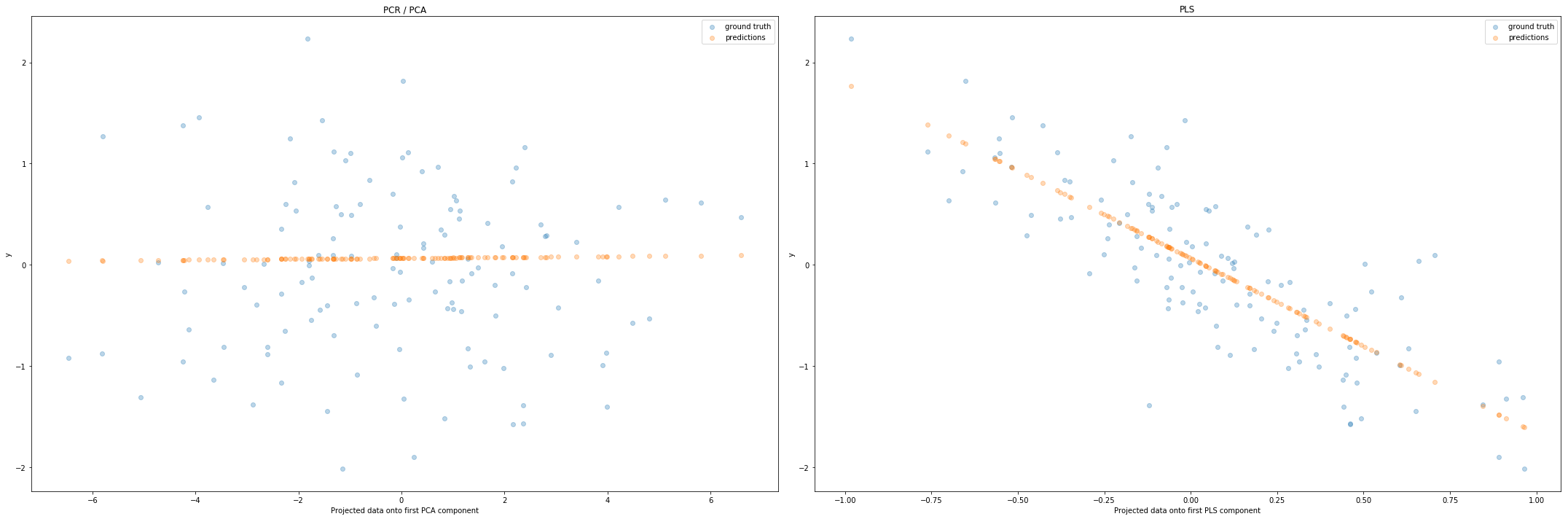
PCA vs PLS

1. PLS는 Y와의 공분산이 높은 k개의 선형조합 변수를 추출하는 방석이다. -> Feature Extraction: ex) $X \in R^{n \times p} \xrightarrow{PLS} X^{‘} \in R^{n \times k} \text{ , s.t. }p < k$
2. PCA와는 다르게 Y와의 상관관계를 반영하는 특징으로서 Supervised feature extraction방법 이다.

2 방법의 차이를 식으로서 나타내면 다음과 같다.

• \(X: \text{Input}, Y: \text{Output}, w: \text{weight}, t = Xw\)

$$\text{cov}(t, Y) = \frac{\text{cov}(t,Y)}{\sqrt{\text{var}(t)}\sqrt{\text{var}(Y)}}\sqrt{\text{var}(t)}\sqrt{\text{var}(Y)} = \text{corr}(t,Y)\sqrt{\text{var}(t)}\sqrt{\text{var}(Y)}$$

$$\text{PLS} = \text{Maximize cov}(t, Y) \propto \text{Maximize corr}(t,Y)\text{var}(t)$$

$$\text{PCA} = \text{Maximize var}(t)$$

PLS식에서 중요하게 봐야하는 것은 \(\text{Maximize corr}(t,Y)\)으로서 X선형결합과 Y의 상관관계를 최대화 하면서 \(\text{var}(t)\)으로서 X선형결합의 분산을 최대와 한다는 것 이다.
즉, Y를 잘 나타낼 수 있는 t를 학습(Supervised)하면서 동시에 t에 PCA를 적용(Unsupervised feature extraction)함으로 인하여, Supervised feature extraction이 가능하다는 것 이다.

from sklearn.model_selection import train_test_split
from sklearn.pipeline import make_pipeline
from sklearn.linear_model import LinearRegression
from sklearn.preprocessing import StandardScaler
from sklearn.decomposition import PCA
from sklearn.cross_decomposition import PLSRegression
import matplotlib.pyplot as plt
import numpy as np

rng = np.random.RandomState(0)
n_samples = 500
cov = [[3, 3],
       [3, 4]]
X = rng.multivariate_normal(mean=[0, 0], cov=cov, size=n_samples)
pca = PCA(n_components=2).fit(X)

y = X.dot(pca.components_[1]) + rng.normal(size=n_samples) / 2

X_train, X_test, y_train, y_test = train_test_split(X, y, random_state=rng)

pcr = make_pipeline(StandardScaler(), PCA(n_components=1), LinearRegression())
pcr.fit(X_train, y_train)
pca = pcr.named_steps['pca']  # retrieve the PCA step of the pipeline

pls = PLSRegression(n_components=1)
pls.fit(X_train, y_train)

fig, axes = plt.subplots(1, 2, figsize=(30, 10))
axes[0].scatter(pca.transform(X_test), y_test, alpha=.3, label='ground truth')
axes[0].scatter(pca.transform(X_test), pcr.predict(X_test), alpha=.3,
                label='predictions')
axes[0].set(xlabel='Projected data onto first PCA component',
            ylabel='y', title='PCR / PCA')
axes[0].legend()
axes[1].scatter(pls.transform(X_test), y_test, alpha=.3, label='ground truth')
axes[1].scatter(pls.transform(X_test), pls.predict(X_test), alpha=.3,
                label='predictions')
axes[1].set(xlabel='Projected data onto first PLS component',
            ylabel='y', title='PLS')
axes[1].legend()
plt.tight_layout()
plt.show()

How to define w

X, Y는 input과 output으로서 주어진 data이므로 weight만 학습하면 된다. PLS에서 weight를 학습하는 식을 적으면 다음과 같다.

$$\text{Object function}: \text{Maximize cov}(t, Y)$$

$$\text{cov}(t, Y) = \text{cov}(Xw, Y) = E[(Xw - E[Xw]) \cdot (Y-E[Y])]$$

$$= E[(Xw) \cdot Y] (\text{mean centering} \rightarrow E[Xw], E[Y] = 0)$$

$$=\frac{1}{n} \sum_{i=1}^{n} (Xw)_i \cdot Y_i = \frac{1}{n} w^T(X^T Y)$$

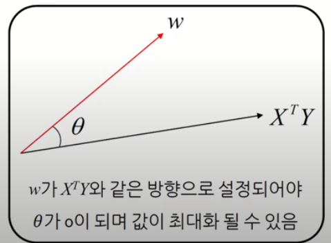
$$\text{cov}(t, Y) \propto \frac{1}{n} w^T(X^T Y) \propto w^T(X^T Y) = \|w\|\cdot\|X^T Y\|\cdot \text{cos}\theta$$

$$\therefore \text{Maximize cov}(t, Y) \propto \text{Maximize} \|w\|\cdot\|X^T Y\|\cdot \text{cos}\theta$$

위의 식에서 X, Y는 주어진 값이고 \(\|w\|\)은 w가 정해지면 변치않는 값이다. 따라서 \(\text{cos}\theta = 1 \rightarrow \theta = 0 \rightarrow w = X^T Y\)인 경우 가장 큰 값을 가지게 될 것이고 이를 사진으로 표현하면 아래와 같다.

PLS - NIPALS Algorithm

위에서 \(\text{PLS} = \text{Maximize cov}(t, Y) \propto \text{Maximize corr}(t,Y)\text{var}(t)\)으로서 식을 나타낼 수 있다고 하였지만, \(\text{Maximize cov}(t, Y) \rightarrow w = X^T Y\)로서 \(\text{Maximize var}(t)\)조건은 빼고 생각하였다. 이러한 조건을 추가하여 계산하는 방식은 NLPALS Algorithm을 통하여 이루워 진다.

Nonlinear Iterative Partial Least Squares (NLPALS) Algorithm

• \(X \in R^{N \times P}: \text{Input}, Y \in R^{N \times 1}: \text{Output}, w \in R^{P \times 1}: \text{weight}, t = Xw \in R^{N \times 1}\)

Step 1. 데이터 정규화 (mean centering)

Step 2. 첫 번째 PLS 변수 (\(t_1\))추출
(1) 첫 번째 \(X_1 = X, Y_1 = Y\)설정

(2) 공분산이 최대가 되도록 하는 선형조합의 가준이 \(w_1\) 계산

• \(w_1 = \frac{X_1^T Y_1}{\|X_1^T Y_1\|} \rightarrow \|w_1\| = 1 \text{ (scaling)}\)

(3) 가중지 \(w_1\)을 이용하여 첫 번째 PLS변수 \(t_1\) 추출

• \(t_1 = X_1 w_1\)

Step3. 두 번째 PLS 변수 (\(t_2\))추출
(1) 두 번째 \(X_2 = X, Y_2 = Y\)설정 앞서 탐색한 \(t_1\)이 설명하지 못하는 부분만을 고려하기 위하여(\(\text{Maximize var}(t)\)), \(t_1\)이 기존 X,Y에 대해서 각각 설명하는 부분을 제외함

(1-1) 변수 \(t_1\)과 회귀계수 \(b_1\)을 사용하여, \(t_1\)이 기존 \(Y_1\)에 대하여 설명하는 부분을 제외

• \(Y_1 = t_1 b_1 + F_1 \rightarrow b_1 = (t_1^T t_1)^{-1}t_1^T Y_1\)
• \(Y_2 = F_1 = Y_1 - t_1 b_1\) , \(F_1 \rightarrow Y_1\)에 대한 잔차(\(t_1\)이 \(Y_1\)에 대해 설명하지 못하는 부분)

(1-2) 변수 \(t_1\)과 회귀계수 \(p_1\)을 사용하여, \(t_1\)이 기존 \(X_1\)에 대하여 설명하는 부분을 제외

• \(X_1 = t_1 p_1 + E_1 \rightarrow p_1^T = (t_1^T t_1)^{-1}t_1^T X_1\)
• \(X_2 = E_1 = X_1 - t_1 p_1^T\), \(E_1 \rightarrow X_1\)에 대한 잔차(\(t_1\)이 \(X_1\)에 대해 설명하지 못하는 부분)

Step4. Step2, 3을 반복하면서 k번째 PLS변수 추출
(1) k 번째 \(X_k = X, Y_k = Y\)설정

(1-1) 변수 \(t_{k-1}\)과 회귀계수 \(b_{k-1}\)을 사용하여, \(t_{k-1}\)이 기존 \(Y_{k-1}\)에 대하여 설명하는 부분을 제외

• \(Y_{k-1} = t_{k-1} b_{k-1} + F_{k-1} \rightarrow b_{k-1} = (t_{k-1}^T t_{k-1})^{-1}t_{k-1}^T Y_{k-1}\)
• $$Y_{k} = F_{k-1} = Y_{k-1} - t_{k-1} b_{k-1}$

(1-2) 변수 \(t_{k-1}\)과 회귀계수 \(p_{k-1}\)을 사용하여, \(t_{k-1}\)이 기존 \(X_{k-1}\)에 대하여 설명하는 부분을 제외

• \(X_{k-1} = t_{k-1} p_{k-1} + E_{k-1} \rightarrow p_{k-1}^T = (t_{k-1}^T t_{k-1})^{-1}t_{k-1}^T X_{k-1}\)
• $$X_{k} = E_{k-1} = X_{k-1} - t_{k-1} p_{k-1}^T$

(2) 공분산이 최대가 되도록 하는 선형조합 가중지 \(w_k\) 계산

• \(w_k = \frac{X_k^T Y_k}{\|X_k^T Y_k\|} \rightarrow \|w_k\| = 1 \text{ (scaling)}\)

(3) 가중지 \(w_k\)을 이용하여 k 번째 PLS변수 \(t_k\) 추출

• \(t_k = X_k w_k\)

Step 5. 충분한 PLS변수가 추출되었으면, 이를 통해 예측 값을 계산

• \(\hat{Y} = \sum_{i+1}^k t_i b_i = \hat{\beta_1}X_1+\hat{\beta_2}X_2+\ldots+\hat{\beta_k}X_k\)

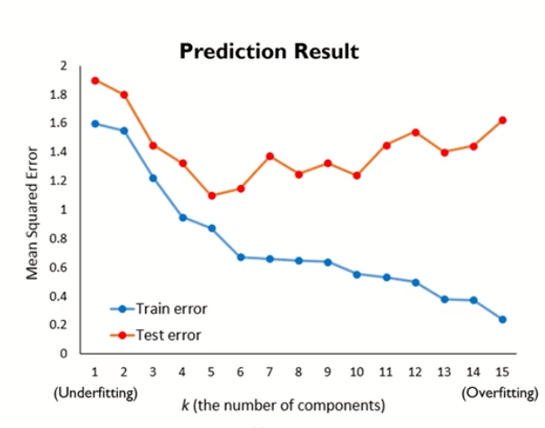
How to define K?
K를 순차적으로 증가시키며 예측 결과를 확인하고, 가장 좋은 예측 결과를 보이는 K를 선택한다. K가 증가될수록 Train Error는 감소되지만, Test Error는 증가되는 Overfitting결과를 보여준다.

PLS - 확장 모델

PLS-DA(Discriminant Analysis): Y가 category value일때의 경우이므로, Y를 one-hot encoding형식 or binary인 경우에는 -1, 1로서 표현한다.

PLS의 출력변수가 여러개여도, 하나의 PLS모델로 여러개의 Y값을 예측가능하다. 하지만, Y에서도 변수를 추출하여야 한다.

$$\text{Maximize cov}(Xw, Y) \xrightarrow{Y \in R^{N \times 1} \rightarrow Y \in R^{N \times M}} \text{Maximize cov}(Xw, Yu)$$

PLS - 확장모델 NLPALS Algorithm

Step 1. 데이터 정규화 (mean centering)

Step 2. PLS 변수 추출
(1) 첫 번째 \(X_1 = X, Y_1 = Y\)설정

(2) 다음 과정을 수렴할 때 까지 반복(\(u\)의 모든 원소값이 이전의 값들과 동일할 때 까지)

(2-1) 임의의 Y변수를 \(u_1\)로 지정한다. (제곱합이 큰 Y변수를 통상적으로 선택)

(2-2) \(u_1\)와의 공분산이 최대가 되는 \(w_1\)계산

• \(w_1 = \frac{X_1^T u_1}{\|X_1^T u+1\|} \rightarrow \|w\| = 1\)

(2-3) \(t_1\) 계산

• \(t_1 = X_1 w_1\)

(2-4) \(X\)에서 추출된 변수 \(t_1\)과의 공분산이 최대가 되는 \(q_1\)계산

• \(q_1 = \frac{Y_1^T t_1}{\|Y_1^T t_1\|} \rightarrow \|q_1\|=1\)

(2-5) \(u_1\)을 계산

• \(u_1 = Y_1 q_1\)

(2-6) (2-1)의 \(u_1\)에 (2-6)을 대입한다.

(3) 변수 \(t_1\)를 \(u_1\)에 대해 회귀분석 후 회귀계수 \(b_1\)을 계산

• \(u_1 = b_1 t_1 + F_1 \rightarrow b_1 = (t_1^T t_1)^{-1} t_1^T u_1\)

Step3. 두 번째 PLS 변수 추출
(1) 두 번째 \(X_2, Y_2\)설정

(1-1) 변수 \(t_1\)과 회귀계수 \(b_1\)을 사용하여, \(t_1\)이 기존 \(Y_1\)에 대하여 설명하는 부분을 제외

• \(u_1 = Y_1 q_1 = b_1 t_1 + F_1 \rightarrow Y_1 q_1 q_1^T = b_1 t_1 q_1^T + F_1 \xrightarrow{\|q\| = q_1 q_1^T = 1} Y_1 = b_1 t_1 q_1^T + F_1\)
• \(Y_2 = F_1 = Y_1 - t_1 b_1 q_1\)

(1-2) 변수 \(t_1\)과 회귀계수 \(p_1\)을 사용하여, \(t_1\)이 기존 \(X_1\)에 대하여 설명하는 부분을 제외

• \(X_1 = t_1 p_1 + E_1 \rightarrow p_1^T = (t_1^T t_1)^{-1}t_1^T X_1\)
• \(X_2 = E_1 = X_1 - t_1 p_1^T\)

Step4. Step2, 3을 반복하면서 k번째 PLS변수 추출

Step 5. 충분한 PLS변수가 추출되었으면, 이를 통해 예측 값을 계산

• \(\hat{Y} = \sum_{i+1}^k b_i t_i q_i^T\)

Example

\(X \in R^{5 \times 3}: \text{Input}, Y\in R^{5 \times 1}: \text{Output}, t = Xw \in R^{5 \times 1}\)

X1 = np.array([-1.1930, -0.0370, -0.5919, 0.3792, 1.4427])
X2 = np.array([-1.0300, -0.7647, -0.3257, 1.0739, 1.0464])
X3 = np.array([1.5012, 0.3540, -0.0910, -0.7140, -1.0502])
X = np.vstack([X1, X2, X3]).T
Y = np.array([-1.1841, -0.2161, -0.5457, 0.5485, 1.3973])

print('Mean X: {:.2f}, Mean Y: {:.2f}'.format(np.mean(X), np.mean(Y)))

Mean X: -0.00, Mean Y: -0.00

1st PLS 변수

• \(X_1 = X, Y_1 = Y\)
• \(w_1 = \frac{X_1^T Y_1}{\|X_1^T Y_1\|}\)
• \(t_1 = X_1 w_1\)

X1 = X
Y1 = Y

w1 = np.dot(X.T, Y)/np.linalg.norm(np.dot(X.T, Y))
t1 = np.dot(X, w1)

print('X1')
print(X1)

print('\nY1')
print(Y1)

print('\nw1')
print(w1)

print('\nt1')
print(t1)

X1
[[-1.193  -1.03    1.5012]
 [-0.037  -0.7647  0.354 ]
 [-0.5919 -0.3257 -0.091 ]
 [ 0.3792  1.0739 -0.714 ]
 [ 1.4427  1.0464 -1.0502]]

Y1
[-1.1841 -0.2161 -0.5457  0.5485  1.3973]

w1
[ 0.61059034  0.55615285 -0.56380266]

t1
[-2.14765227 -0.64746807 -0.49124136  1.2313435   2.05496258]

2nd PLS 변수

• \(b_1 = (t_1^T t_1)^{-1}t_1^T Y_1 \rightarrow Y_2 = Y_1 - t_1 b_1\)
• \(p_1 = (t_1^T t_1)^{-1}t_1^T X_1 \rightarrow X_2 = X_1 - t_1 p_1\)
• \(w_2 = \frac{X_2^T Y_2}{\|X_2^T Y_2\|}, t_2 = X_2 w_2\)

b1 = np.dot((np.dot((1/np.dot(t1.transpose(), t1)), t1.transpose())), Y1)
p1 = np.dot((np.dot((1/np.dot(t1.transpose(), t1)), t1.transpose())), X1)

X2 = X1-np.dot(t1.reshape(-1,1), p1.reshape(-1,1).transpose())
Y2 = Y1-np.dot(t1.reshape(-1,1), b1.reshape(-1,1)).reshape(Y.shape)

w2 = np.dot(X2.T, Y2)/np.linalg.norm(np.dot(X2.T, Y2))
t2 = np.dot(X2, w2)

print('X2')
print(X2)

print('\nY2')
print(Y2)

print('\nw2')
print(w2)

print('\nt2')
print(t2)

X2
[[ 0.0373323   0.20644826  0.24407747]
 [ 0.33391707 -0.39193911 -0.02499371]
 [-0.31048102 -0.04288209 -0.37854682]
 [-0.32620362  0.36498983  0.00676364]
 [ 0.26546713 -0.13668487  0.15266687]]

Y2
[ 0.08315563  0.16594861 -0.25583539 -0.17807339  0.18473736]

w2
[ 0.79169572 -0.41073903  0.45222929]

t2
[ 0.05513845  0.41404252 -0.39938311 -0.40511087  0.33535143]

3rd PLS 변수

• \(b_2 = (t_2^T t_2)^{-1}t_2^T Y_2 \rightarrow Y_3 = Y_2 - t_2 b_2\)
• \(p_2 = (t_2^T t_2)^{-1}t_2^T X_2 \rightarrow X_3 = X_2 - t_2 p_2\)
• \(w_3 = \frac{X_3^T Y_3}{\|X_3^T Y_3\|}, t_3 = X_3 w_3\)

b2 = np.dot((np.dot((1/np.dot(t2.transpose(), t2)), t2.transpose())), Y2)
p2 = np.dot((np.dot((1/np.dot(t2.transpose(), t2)), t2.transpose())), X2)

X3 = X2-np.dot(t2.reshape(-1,1), p2.reshape(-1,1).transpose())
Y3 = Y2-np.dot(t2.reshape(-1,1), b2.reshape(-1,1)).reshape(Y.shape)

w3 = np.dot(X3.T, Y3)/np.linalg.norm(np.dot(X3.T, Y3))
t3 = np.dot(X3, w3)

print('X3')
print(X3)

print('\nY3')
print(Y3)

print('\nw3')
print(w3)

print('\nt3')
print(t3)

X3
[[-0.00651165  0.2360216   0.22576718]
 [ 0.00468654 -0.16986865 -0.16248837]
 [ 0.00709291 -0.25709002 -0.24592023]
 [-0.0040752   0.14770984  0.14129229]
 [-0.0011913   0.04317986  0.04130383]]

Y3
[ 0.05519936 -0.04397899 -0.0533404   0.02732569  0.01470768]

w3
[-0.01993285  0.72248699  0.69109712]

t3
[ 0.32667938 -0.23511655 -0.35584034  0.20444636  0.05976559]

• \(b_3 = (t_3^T t_3)^{-1}t_3^T Y_3\)
• \(p_3 = (t_3^T t_3)^{-1}t_3^T X_3\)

Prediction Y
\(\hat{Y} = \sum_{i+1}^k t_i b_i\)

if k = 1

b3 = np.dot((np.dot((1/np.dot(t3.transpose(), t3)), t3.transpose())), Y3)
p3 = np.dot((np.dot((1/np.dot(t3.transpose(), t3)), t3.transpose())), X3)

y_hat = np.dot(t1, b1)

print('Label: ', Y)
print('\nPrediction: ', y_hat)
print('\nMSE Loss: {:.4f}'.format(np.mean((Y-y_hat)**2)))

Label:  [-1.1841 -0.2161 -0.5457  0.5485  1.3973]

Prediction:  [-1.26725563 -0.38204861 -0.28986461  0.72657339  1.21256264]

MSE Loss: 0.0331

if k = 2

y_hat = np.dot(t1, b1) + np.dot(t2, b2)

print('Label: ', Y)
print('\nPrediction: ', y_hat)
print('\nMSE Loss: {:.4f}'.format(np.mean((Y-y_hat)**2)))

Label:  [-1.1841 -0.2161 -0.5457  0.5485  1.3973]

Prediction:  [-1.23929936 -0.17212101 -0.4923596   0.52117431  1.38259232]

MSE Loss: 0.0018

if k = 3

y_hat = np.dot(t1, b1) + np.dot(t2, b2) + np.dot(t3, b3)

print('Label: ', Y)
print('\nPrediction: ', y_hat)
print('\nMSE Loss: {:.4f}'.format(np.mean((Y-y_hat)**2)))

Label:  [-1.1841 -0.2161 -0.5457  0.5485  1.3973]

Prediction:  [-1.18665868 -0.21000738 -0.54969924  0.55411853  1.39222287]

MSE Loss: 0.0000

---

참조: YouTube: 핵심 머신러닝-Partial Least Square(PLS)

코드에 문제가 있거나 궁금한 점이 있으면 wjddyd66@naver.com으로 Mail을 남겨주세요.