OpenCV-영상 공간 필터링

25 minute read

참고사항
현재 Post에서 사용하는 Data를 만드는 법이나 사용한 Image는 github에 올려두었습니다.

영상 공간 필터링

이미지 필터링(image filtering)은 필터(filter) 또는 커널(kernel) 또는 윈도우(window)라고 하는 정방행렬을 정의하고 이 커널은 이동시키면서 같은 임미지 영역과 곱하여 그 결과값을 이미지의 해당 위치의 값으로 하는 새로운 이미지를 만드는 연산이다.
기호 $\otimes$로 표기한다.

원본 이미지의 화소(x,y)의 위치의 명도를 f(x,y)를 필터이미지 h(x,y), 필터링된 결과를 g(x,y)라고 하면 수식은 다음과 같다.

$$f \otimes h = \sum_{u=-K/2}^{K} \sum_{u=-K/2}^{K} f(x+u,y+v) \cdot h(u,v)$$

위의 식에서 K는 필터 크기의 절반을 의미한다. ex) 3 x 3 크기의 필터에서는 K=1이다.
만약 위의 식에서 필터를 좌우 상하를 뒤집으면 콘볼루션(convolution)이라고 한다. 기호고는 $*$로서 표기한다.

$$f * h = \sum_{u=-K/2}^{K} \sum_{u=-K/2}^{K} f(x-u,y-v) \cdot \tilde{h}(u,v)$$

$$\tilde{h}(u,v) = h(-u,-v)$$

사진 출처:데이터 사이언스 스쿨

블러필터

영상을 부드럽게 하는 블러링(bluring)/스무딩(smoothing)필터를 사용하게되면 영상의 잡음(noise)를 제거하고 영상을 부드럽게 한다.
이러한 필터들은 고주파의 성분들을 저주파의 성분들로 근사시키는 역할을 하므로 LPF(Low Pass Filter)라고 불린다.

cv2.boxFilter(src, ddepth, ksize[, dst[, anchor[, normalize[, borderType]]]]): 균일한 값을 가지는 커널을 이용한 이미지 필터링이다. 커널 영역내의 평균값으로 해당 픽셀을 대체한다.
parameter

src: input
ddepth: outputimage depth
ksize: bluring kernel size
anchor: 커널 중심, default: (-1,-1)
normalize: flag, 정규화
borderType: padding방법

식

$$K=\alpha \begin{bmatrix} 1 & 1 & 1 & ... & 1 \\ 1 & 1 & 1 & ... & 1 \\ & & ... & & \\ 1 & 1 & 1 & ... & 1 \end{bmatrix}$$

$$ \alpha = \begin{cases} \frac{1}{kw x kh} & \mbox{if } normalize=True \\ 1 & \mbox{else} \end{cases} $$

cv2.blur(src, ksize[, dst[, anchor[, borderType]]]) : Box Filter에서 normalized=True한 Filter이다.

cv2.medianBlur(src, ksize[, dst]) : 평균값이 아닌 중앙값으로 픽셀값을 바꾸는 방법이다. 점 모양의 잡음을 제거하는데 효과적인다

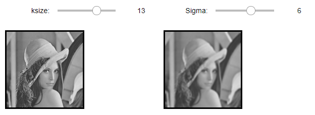
cv2.GaussianBlur(src, ksize, sigmaX[, dst[, sigmaY[, borderType]]]): 필터를 가우시안 Kernel과 Convolution을 수행한다.
가우시안 필터는 순환 대칭, 단일 돌출(Single peak)부분을 가진다. 즉, 중앙에 위치한 pixel과 먼 pixel값들을 낮추는 효과로서 잡음제거 효과가 있다.
참고사항: 가우시안 필터
parameter

sigmaX : X-축 방향으로 가우시안 커널 표준편차
sigmaY: Y-축 방향으로 가우시안 커널 표준편차

$$ sigmaX = sigmaY (\text{if } sigmaX \neq 0, sigmaY \neq 0)$$

$$ sigmaX = 0.3(((kw-1)/2)-1)+0.8 (\text{if } sigmaX = 0$$

$$ sigmaY = 0.3(((kh-1)/2)-1)+0.8 (\text{if } sigmaY = 0$$

식

$$f \otimes G = \sum_{u=-K/2}^{K} \sum_{u=-K/2}^{K} f(x+u,y+v) \cdot G(u,v)$$

$$= \sum_{u=-K/2}^{K} \sum_{u=-K/2}^{K} f(x+u,y+v) \cdot G((x+u)-x,(y+v)-v)$$

cv2.bilateralFilter(src, d, sigmaColor, sigmaSpace[, dst[, borderType]]): 위에서 설명한 가우시안 필터를 사용하게 되면 이미지의 경계선을 무시하는 블러 필터 이다. 하지만 양방향 필터링을 사용하게 되면, 두 픽셀과의 거리 뿐 아니라 두 픽셀의 명앖값의 차이도 커널에 넣어서 가중치로 곱한다.

식

$$ \begin{multline} f \otimes G = \\ \sum_{u=-K/2}^{K} \sum_{u=-K/2}^{K} (f(x+u,y+v) \cdot \\ G((x+u)-x,(y+v)-v) \cdot \\ G^{\prime}(f(x+u)-f(x),f(y+v)-f(v))) \end{multline} $$

추가사항: borderType(ksize=3)인 경우

bordertype	왼쪽패딩	배열	왼쪽패딩
cv2.BORDER_CONSTANT	000	123456	000
cv2.BORDER_REPLICATE	111	123456	111
cv2.BORDER_REFLECT	321	123456	654
cv2.BORDER_REFLECT_101	234	123456	543
cv2.BORDER_WRAP	456	123456	123

#Component 선언
IntSlider_Box = IntSlider(
    value=1,
    min=1,
    max=30,
    step=1,
    description='ksize: ',
    disabled=False,
    continuous_update=False,
    orientation='horizontal',
    readout=True,
    readout_format='d'
)

IntSlider_Biateral = IntSlider(
    value=0,
    min=-1,
    max=30,
    step=1,
    description='d: ',
    disabled=False,
    continuous_update=False,
    orientation='horizontal',
    readout=True,
    readout_format='d'
)

IntSlider_MedianBlur = IntSlider(
    value=1,
    min=1,
    max=20,
    step=2,
    description='ksize: ',
    disabled=False,
    continuous_update=False,
    orientation='horizontal',
    readout=True,
    readout_format='d'
)


IntSlider_Blur = IntSlider(
    value=1,
    min=1,
    max=20,
    step=1,
    description='ksize: ',
    disabled=False,
    continuous_update=False,
    orientation='horizontal',
    readout=True,
    readout_format='d'
)

IntSlider_Gaussian = IntSlider(
    value=1,
    min=1,
    max=20,
    step=2,
    description='ksize: ',
    disabled=False,
    continuous_update=False,
    orientation='horizontal',
    readout=True,
    readout_format='d'
)

IntSlider_Gaussian2 = IntSlider(
    value=0,
    min=0,
    max=10,
    step=1,
    description='Sigma: ',
    disabled=False,
    continuous_update=False,
    orientation='horizontal',
    readout=True,
    readout_format='d'
)

def layout(header, left, right):
    layout = AppLayout(header=header,
          left_sidebar=left,
          center=None,
          right_sidebar=right)
    return layout

wImg_original = Image(layout = Layout(border="solid"), width="50%") 
wImg_Box = Image(layout = Layout(border="solid"), width="50%") 
wImg_Biateral = Image(layout = Layout(border="solid"), width="50%") 
wImg_MedianBlur = Image(layout = Layout(border="solid"), width="50%") 
wImg_Blur = Image(layout = Layout(border="solid"), width="50%") 
wImg_Gaussian = Image(layout = Layout(border="solid"), width="50%") 

box1 = layout(IntSlider_Box,wImg_original,wImg_Box)
box2 = layout(IntSlider_Biateral,wImg_original,wImg_Biateral)
box3 = layout(IntSlider_MedianBlur,wImg_original,wImg_MedianBlur)
box4 = layout(IntSlider_Blur,wImg_original,wImg_Blur)

items = [IntSlider_Gaussian,IntSlider_Gaussian2]
Gaussian = Box(items)
box5 = layout(Gaussian,wImg_original,wImg_Gaussian)


tab_nest = widgets.Tab()
tab_nest.children = [box1, box2, box3, box4, box5]
tab_nest.set_title(0, 'Box Filter')
tab_nest.set_title(1, 'Biateral Filter')
tab_nest.set_title(2, 'MedianBlur Filter')
tab_nest.set_title(3, 'Blur Filter')
tab_nest.set_title(4, 'Gaussian Filter')
tab_nest

img = cv2.imread('./data/lena.jpg',0)
tmpStream = cv2.imencode(".jpeg", img)[1].tostring()
wImg_original.value = tmpStream

display.display(tab_nest)

#Event 선언
gaussian_ksize, gaussian_sigma = 1,0

def on_value_change_Box(change):
    ksize = change['new']
    Box_img = cv2.boxFilter(img,ddepth=-1,ksize=(ksize,ksize))
    tmpStream = cv2.imencode(".jpeg", Box_img)[1].tostring()
    wImg_Box.value = tmpStream
    
def on_value_change_Biateral(change):
    d = change['new']
    Biateral_img = cv2.bilateralFilter(img,d=d,sigmaColor = 10, sigmaSpace = 10)
    tmpStream = cv2.imencode(".jpeg", Biateral_img)[1].tostring()
    wImg_Biateral.value = tmpStream
    
def on_value_change_MedianBlur(change):
    ksize = change['new']
    MedianBlur_img = cv2.medianBlur(img,ksize=ksize)
    tmpStream = cv2.imencode(".jpeg", MedianBlur_img)[1].tostring()
    wImg_MedianBlur.value = tmpStream
    
def on_value_change_Blur(change):
    ksize = change['new']
    Blurr_img = cv2.blur(img,ksize=(ksize,ksize))
    tmpStream = cv2.imencode(".jpeg", Blurr_img)[1].tostring()
    wImg_Blur.value = tmpStream
    
def on_value_change_Gaussian(change):
    global gaussian_ksize, gaussian_sigma
    gaussian_ksize = change['new']
    Gaussian_img = cv2.GaussianBlur(img,ksize=(gaussian_ksize,gaussian_ksize),sigmaX=gaussian_sigma)
    tmpStream = cv2.imencode(".jpeg", Gaussian_img)[1].tostring()
    wImg_Gaussian.value = tmpStream
    
def on_value_change_Gaussian2(change):
    global gaussian_ksize, gaussian_sigma
    gaussian_sigma = change['new']
    Gaussian_img = cv2.GaussianBlur(img,ksize=(gaussian_ksize,gaussian_ksize),sigmaX=gaussian_sigma)
    tmpStream = cv2.imencode(".jpeg", Gaussian_img)[1].tostring()
    wImg_Gaussian.value = tmpStream
    

#초기화 작업
Box_img = cv2.boxFilter(img,ddepth=-1,ksize=(1,1))
tmpStream = cv2.imencode(".jpeg", Box_img)[1].tostring()
wImg_Box.value = tmpStream

Biateral_img = cv2.bilateralFilter(img,d=0,sigmaColor = 10, sigmaSpace = 10)
tmpStream = cv2.imencode(".jpeg", Biateral_img)[1].tostring()
wImg_Biateral.value = tmpStream
    
MedianBlur_img = cv2.medianBlur(img,ksize=1)
tmpStream = cv2.imencode(".jpeg", MedianBlur_img)[1].tostring()
wImg_MedianBlur.value = tmpStream

Blurr_img = cv2.blur(img,ksize=(1,1))
tmpStream = cv2.imencode(".jpeg", Blurr_img)[1].tostring()
wImg_Blur.value = tmpStream

Gaussian_img = cv2.GaussianBlur(img,ksize=(gaussian_ksize,gaussian_ksize),sigmaX=gaussian_sigma)
tmpStream = cv2.imencode(".jpeg", Gaussian_img)[1].tostring()
wImg_Gaussian.value = tmpStream

#Component에 Event 장착
IntSlider_Box.observe(on_value_change_Box, names='value')
IntSlider_Biateral.observe(on_value_change_Biateral, names='value')
IntSlider_MedianBlur.observe(on_value_change_MedianBlur, names='value')
IntSlider_Blur.observe(on_value_change_Blur, names='value')
IntSlider_Gaussian.observe(on_value_change_Gaussian, names='value')
IntSlider_Gaussian2.observe(on_value_change_Gaussian2, names='value')

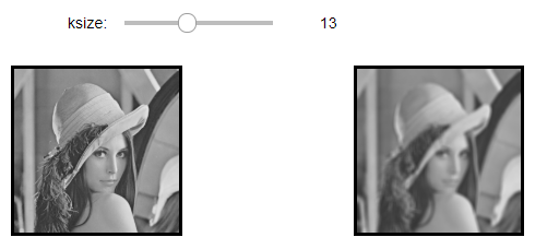
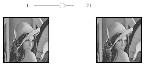
블러 필터 결과
Box Filter(ksize = 13)

Biateral Filter(d = 21)

Median Blur Filter(ksize = 50)

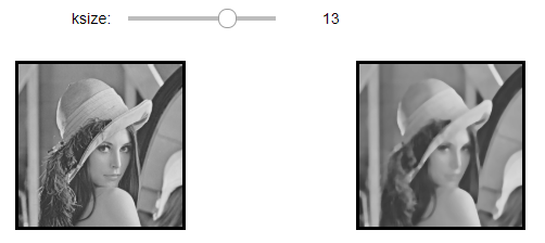
Blur Filter(ksize = 13)

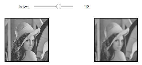
Gaussian Filter(ksize = 13, sigma=6)

미분필터

미분필터란 영상내의 여러가지 정보중 특별히 feature라고 명칭하는, 영상이 가지는 특별한 정보들이 있다.
이러한 feature의 기본적인 요소로 blob, corner, edge등이 존재하게 된다.
corner, edge의 경우 자신을 경계로하여 주변의 밝기값이 급격하게 변화하는 현상을 보이기 때문에 고주파 성분에 해당한다.
이러한 고주파 성분을 찾아내는 필터이기 때문에 HPF(High Pass Filter)라고 불리게 된다.

미분 연산
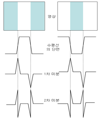
1차 미분
함수 f(x)에서 1차미분, $f^{\prime}(x)$는 다음과 같이 나타낼 수 있다.

$$f^{\prime}(x) = \frac{\partial f(x)}{\partial x} = \lim_{h \rightarrow 0} \frac{f(x+h)-f(x)}{h}$$

위의 식을 Image로적용시키면 h는 0에 가까워질수 없고 최소로 작은수는 인접화소를 가르킬수 있는 1의 값을 가지게 된다.
이러한 Image의 특성을 고려하면 최종적인 미분식은 다음과 같다.

$$f^{\prime}(x) = f(x+1) - f(x)$$

2차 미분
위의 식을 활용하여 2차미분식을 유도하면 다음과 같다.

$$f^{\prime \prime}(x) = (f^{\prime}(x))^{\prime} = (f(x+1) - f(x))^{\prime}$$

$$= \frac{\partial(f(x+1)-f(x))}{\partial x} = \frac{\partial f(x+1)}{\partial x} - \frac{\partial f(x)}{\partial x}$$

$$= \lim_{h \rightarrow 0} \frac{f(x+1+h)-f(x+1)}{h} - \lim_{h \rightarrow 0} \frac{f(x+h)-f(x)}{h}$$

$$= f(x+2) - f(x+1) - f(x+1) + f(x) $$

$$= f(x+2) - 2f(x+1) + f(x)$$

$$\therefore f^{\prime \prime}(x) = f(x+1) - 2f(x) + f(x-1)$$

Sobel Filter
cv2.Sobel(src, ddepth, dx, dy[, dst[, ksize[, scale[, delta[, borderType]]]]]): 지정한 축방향으로의 디지털 형태의 미분을 구현. 1차미분을 통하여 특정한 Edge를 검출하는 Filter이다.

parameter

src: input
ddept: output image depth
dx: x에 대한 미분 차수
dy: y에 대한 미분 차수
ksize: Sobel kernel 크기 (1,3,5,7만 가능)

example

사진 출처:bskyvision 블로그

수직엣지 검출을 살펴보게 되면 위에서 정리한 식(1차 미분) $f^{\prime}(x) = f(x+1) - f(x)$을 사용한 것을 알 수 있다.
주방향으로는 1이아닌 2의 가중치를 부여하여 Kernel을 구성한다.

Laplacian Filter
cv2.Laplacian(src, ddepth[, dst[, ksize[, scale[, delta[, borderType]]]]]): 1차 미분을 사용하는 Sobel Filter에 비하여 영상내에 blob이나, 섬세한 부분을 더 잘 검출하는 경향을 보인다. 이러한 특징 때문에 2차 미분은 주로 영상개선에 사용하며 1차 미분은 특징검출에 사용된다.

example(3 x 3, ksize=1)

$$\begin{bmatrix} 0 & 1 & 0 \\ 1 & -4 & 1 \\ 0 & 1 & 0 \end{bmatrix}$$

위의 식을 살펴보게 되면 위에서 정리한 식(2차 미분) $f^{\prime \prime}(x) = f(x+1) - 2f(x) + f(x-1)$ 을 사용하는 것을 알 수 있다.
각각 x,y에 대하여 미분해야 하므로 식을 바꿔서 정리하면 다음과 같이 나타낼 수 있다.

$$f^{\prime \prime}(x,y) $$

$$= f(x-1,y) + f(x,y-1)$$

$$+ f(x+1,y) + f(x,y+1) - 4f(x,y)$$

주의사항

사진 출처: WORLD of NEO 블로그
위의 사진을 보게되면 Laplacian Filter의 몇가지 특징이 나타나게 된다.

2차미분 방식을 이용하여 영상에서 에지를 검출하면 영상에 대해서 미분을 두 번 수행하기 때문에 에지가 중심 방향에 가능게 형성되며 검출된 윤각선이 폐곡선을 이루게된다.
2차 미분은 밝기 값이 점차적으로 변화되는 영역에 대해서는 반응을 보이지 않는다.
Laplacian Filter는 잡음에 민감하다.

위의 특징으로 인하여 다음과 같은 과정을 거친 뒤 Laplacian Filter를 사용하는 것이 권고된다.
잡음에 민감한 특징
Laplacian Filter를 사용하게 되면 잡음에 민감하다는 것때문에 Gausian Filter를 통하여 Smoothing및 잡음 제거 후 Laplacian Filter를 사용하게 된다.
폐곡선
폐곡선의 장점은 에지 주변에서 부호가 바뀌게 된다는 것 이다.이러한 부호의 변화를 영교차(zero crossing)이라고 한다.
이러한 zerocrossing을 사용하여 edge 크기를 비교하여 임계값 이상일 경우에 에지로 정의할 수 있도록 임의의 임계값을 활용하여 edge를 출력할 수 있다.

참고사항1(magnitude)
cv2.magnitude(x, y[, magnitude]) : 2D vector의 magnitude계산
parameter

x: floating point1
y: floating point2
manitude: $dst = \sqrt{x^2+y^2}$

참고사항2(각도 계산)
sobel filter를 통하여 x와 y에 관한 각각의 미분값을 얻을 수 있다.
이러한 미분값을 통하여 삼각함수를 이용하여 각도 ($\theta$ )를 계산할 수 있다.

gx: x에 관한 미분값
gy: y에 관한 미분값

$$\theta = tan^{-1}(\frac{gy}{gx})$$

참고 사항3(Normalization)
Local Maxima를 선택하는 단계이다.
극 값을 선택하는데 있어서 잘못된 영역이 나올 수 있다.
즉 진짜 Edge가 아님에도 불구하고 검출이 된 영역이 있다는 것 이다.
이러한 이유는 개인적으로 크게 2가지로 생각한다.

Image의 경우 Text와 달리 주변 pixel끼리의 값이 비슷한 Data의 값이 연속적이라는 특징을 가지고 있기 때문이다.
Blur를 통하여 흐려진 Edge에서 잘못된 검출이 발생하기 때문에 다시 Sharp한 edge로 변환해야 한다.

이러한 Local Maxima는 양 방향과 음 방향으로 에지 강도와 현재 픽셀의 에지 강도를 비교판단을 하여 나타낼 수 있다.
아래 사진은 주변 pixel 4개를 선택하였을때 Local Maxima를 선택하는 예시이다.

사진 출처:carstart 블로그

cv2.normalize(src[, dst[, alpha[, beta[, norm_type[, dtype[, mask]]]]]])
parameter

src: input
alpha: norm value to normalize to or the lower range boundary
beta: upper range boundary
normType: normalization type

Sobel Filter1

src = cv2.imread('./data/rectangle.jpg',cv2.IMREAD_GRAYSCALE) 

gx = cv2.Sobel(src,cv2.CV_32F,1,0,ksize=3)
gy = cv2.Sobel(src,cv2.CV_32F,0,1,ksize=3)

dstX = cv2.sqrt(np.abs(gx))
dstX = cv2.normalize(dstX,None,0,255,cv2.NORM_MINMAX,dtype=cv2.CV_8U)

dstY = cv2.sqrt(np.abs(gy))
dstY = cv2.normalize(dstY,None,0,255,cv2.NORM_MINMAX,dtype=cv2.CV_8U)

mag = cv2.magnitude(gx,gy)
minVal, maxVal, minLoc, maxLoc = cv2.minMaxLoc(mag)
print('mag:',minVal,maxVal,minLoc,maxLoc)
dstM = cv2.normalize(mag,None,0,255,cv2.NORM_MINMAX,dtype=cv2.CV_8U)

plt.figure(figsize=(20,4))
imgae1=plt.subplot(1,4,1)
imgae1.set_title('Original')
plt.axis('off')
plt.imshow(src, cmap="gray")

imgae2=plt.subplot(1,4,2)
imgae2.set_title('dstX')
plt.axis('off')
plt.imshow(dstX, cmap="gray")

imgae3=plt.subplot(1,4,3)
imgae3.set_title('dstY')
plt.axis('off')
plt.imshow(dstY, cmap="gray")

imgae3=plt.subplot(1,4,4)
imgae3.set_title('dstM')
plt.axis('off')
plt.imshow(dstM, cmap="gray")

plt.show()

Sobel Filter1 결과
mag: 0.0 1080.467529296875 (0, 0) (100, 400)

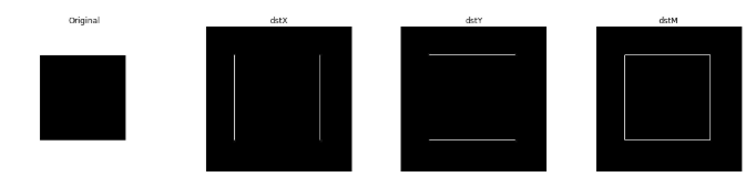
실행 결과 각각의 x,y,xy축으로 미분값(Edge)를 추출하는 것을 알 수 있다.
mag같은 경우 x, y축으로 미분값의 공통된 점으로서 코너점을 출력하는 것을 알 수 있다.

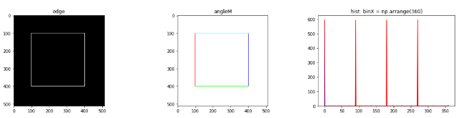
Sobel Filter2(gradient orientation)

cv2.cartToPolar(x, y[, magnitude[, angle[, angleInDegrees]]])는 2D vector의 magnitude계산및 각도도 Return하는 함수이다.
결과 angleM에서 색깔은 각각의 의미와 같다.

빨강: magnitude의 값 중 angle = 0 인곳
초록: magnitude의 값 중 angle = 90 인곳
파랑: magnitude의 값 중 angle = 180 인곳
노랑: magnitude의 값 중 angle = 270 인곳

src = cv2.imread('./data/rectangle.jpg',cv2.IMREAD_GRAYSCALE)

gx = cv2.Sobel(src,cv2.CV_32F,1,0,ksize=3)
gy = cv2.Sobel(src,cv2.CV_32F,0,1,ksize=3)

mag,angle = cv2.cartToPolar(gx,gy,angleInDegrees =True)
minVal,maxVal,minLoc,maxLoc = cv2.minMaxLoc(angle)
print('angle: ',minVal,maxVal,minLoc,maxLoc)

ret,edge = cv2.threshold(mag,100,255,cv2.THRESH_BINARY)
edge = edge.astype(np.uint8)

width,height = mag.shape[:2]
angleM = np.full((width,height,3),(255,255,255),dtype=np.uint8)
for y in range(height):
    for x in range(width):
        if edge[y,x]!=0:
            if angle[y,x] == 0:
                angleM[y,x] = (0,0,255) # red
            elif angle[y,x] == 90:
                angleM[y,x] = (0,255,0) # green
            elif angle[y,x] == 180:
                angleM[y,x] = (255,0,0) # blue
            elif angle[y,x] == 270:
                angleM[y,x] = (0,255,255) # yellow
            else:
                angleM[y,x] = (128,128,128) # gray

hist = cv2.calcHist(images=[angle],channels=[0],mask=edge,histSize=[360],ranges=[0,360])
hist = hist.flatten()
                
plt.figure(figsize=(20,4))
imgae1=plt.subplot(1,3,1)
imgae1.set_title('edge')
plt.imshow(edge, cmap="gray")

imgae2=plt.subplot(1,3,2)
imgae2.set_title('angleM')
plt.imshow(angleM)

imgae3=plt.subplot(1,3,3)
imgae3.set_title('hist: binX = np.arrange(360)')
plt.plot(hist,color='r')
binX=np.arange(360)
plt.bar(binX,hist,width=1,color='b')

plt.show()

Sobel Filter 2 결과
angle: 0.0 359.94378662109375 (0, 0) (400, 399)

Laplacian 필터

원본 이미지를 부드럽게하여 미분 오차를 줄이기 위하여 ksize=(7,7)크기의 필터를 사용한 가우시안 블러링으로 blur를 생성한다.
blur에 라플라시안 필터링을하여 lap을 생성한다.
dst는 lap을 범위[0,255]로 정규화한 결과이다.

#Component 선언
IntSlider_Gaussian = IntSlider(
    value=1,
    min=1,
    max=20,
    step=2,
    description='ksize: ',
    disabled=False,
    continuous_update=False,
    orientation='horizontal',
    readout=True,
    readout_format='d'
)

IntSlider_Gaussian2 = IntSlider(
    value=0,
    min=0,
    max=10,
    step=1,
    description='Sigma: ',
    disabled=False,
    continuous_update=False,
    orientation='horizontal',
    readout=True,
    readout_format='d'
)

def layout(header, left, right):
    layout = AppLayout(header=header,
          left_sidebar=left,
          center=None,
          right_sidebar=right)
    return layout

wImg_original = Image(layout = Layout(border="solid"), width="50%")
wImg_Gaussian = Image(layout = Layout(border="solid"), width="50%")
wImg_Laplacian = Image(layout = Layout(border="solid"), width="50%")
wImg_Laplacian2 = Image(layout = Layout(border="solid"), width="50%")

items = [IntSlider_Gaussian,IntSlider_Gaussian2]
items2 = [wImg_original,wImg_Gaussian]
items3 = [wImg_Laplacian,wImg_Laplacian2]
Gaussian = Box(items)
Input =Box(items2)
Output = Box(items3)
box = layout(Gaussian,Input,Output)


tab_nest = widgets.Tab()
tab_nest.children = [box]
tab_nest.set_title(0, 'Gaussian Filter, Laplacian')
tab_nest

img = cv2.imread('./data/lena.jpg',0)
tmpStream = cv2.imencode(".jpeg", img)[1].tostring()
wImg_original.value = tmpStream

display.display(tab_nest)

#Event 선언
gaussian_ksize, gaussian_sigma = 1,0
    

def on_value_change_Gaussian(change):
    global gaussian_ksize, gaussian_sigma
    gaussian_ksize = change['new']
    Gaussian_img = cv2.GaussianBlur(img,ksize=(gaussian_ksize,gaussian_ksize),sigmaX=gaussian_sigma)
    tmpStream = cv2.imencode(".jpeg", Gaussian_img)[1].tostring()
    wImg_Gaussian.value = tmpStream
    
    make_laplacian(Gaussian_img)
    
def on_value_change_Gaussian2(change):
    global gaussian_ksize, gaussian_sigma
    gaussian_sigma = change['new']
    Gaussian_img = cv2.GaussianBlur(img,ksize=(gaussian_ksize,gaussian_ksize),sigmaX=gaussian_sigma)
    tmpStream = cv2.imencode(".jpeg", Gaussian_img)[1].tostring()
    wImg_Gaussian.value = tmpStream
    
    make_laplacian(Gaussian_img)

def make_laplacian(img):
    lap = cv2.Laplacian(img,cv2.CV_32F)
    minVal,maxVal,minLoc,maxLoc = cv2.minMaxLoc(lap)
    dst = cv2.convertScaleAbs(lap)
    dst = cv2.normalize(dst,None,0,255,cv2.NORM_MINMAX)
    
    lap = lap.astype(np.uint8)
    tmpStream = cv2.imencode(".jpeg", lap)[1].tostring()
    wImg_Laplacian.value = tmpStream
    tmpStream = cv2.imencode(".jpeg", dst)[1].tostring()
    wImg_Laplacian2.value = tmpStream

#초기화 작업
Gaussian_img = cv2.GaussianBlur(img,ksize=(gaussian_ksize,gaussian_ksize),sigmaX=gaussian_sigma)
tmpStream = cv2.imencode(".jpeg", Gaussian_img)[1].tostring()
wImg_Gaussian.value = tmpStream

make_laplacian(Gaussian_img)


#Component에 Event 장착
IntSlider_Gaussian.observe(on_value_change_Gaussian, names='value')
IntSlider_Gaussian2.observe(on_value_change_Gaussian2, names='value')

Laplacian 필터1 결과(ksize=7, sigma=4)

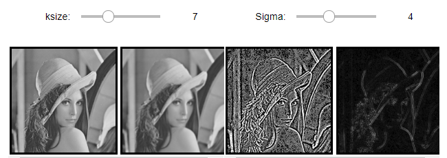
Laplacian 필터2: zero-crossing

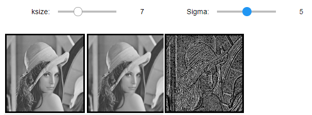
zerocrossing을 사용하여 edge 크기를 비교하여 임계값 이상일 경우에 에지로 정의할 수 있도록 임의의 임계값을 활용하여 edge를 출력할 수 있다.
이러한 결과로 인하여 잡음에 덜 민감한 Laplacian Filter를 적용할 수 있다는 장점이 생기게 된다.

#Component 선언
IntSlider_Gaussian = IntSlider(
    value=1,
    min=1,
    max=20,
    step=2,
    description='ksize: ',
    disabled=False,
    continuous_update=False,
    orientation='horizontal',
    readout=True,
    readout_format='d'
)

IntSlider_Gaussian2 = IntSlider(
    value=0,
    min=0,
    max=10,
    step=1,
    description='Sigma: ',
    disabled=False,
    continuous_update=False,
    orientation='horizontal',
    readout=True,
    readout_format='d'
)

IntSlider_Gaussian3 = IntSlider(
    value=1,
    min=1,
    max=20,
    step=2,
    description='ksize: ',
    disabled=False,
    continuous_update=False,
    orientation='horizontal',
    readout=True,
    readout_format='d'
)

IntSlider_Gaussian4 = IntSlider(
    value=0,
    min=0,
    max=10,
    step=1,
    description='Sigma: ',
    disabled=False,
    continuous_update=False,
    orientation='horizontal',
    readout=True,
    readout_format='d'
)

def layout(header, left, right):
    layout = AppLayout(header=header,
          left_sidebar=left,
          center=None,
          right_sidebar=right)
    return layout

wImg_original = Image(layout = Layout(border="solid"), width="50%") 
wImg_Blur = Image(layout = Layout(border="solid"), width="50%") 
wImg_Gaussian = Image(layout = Layout(border="solid"), width="50%") 

wImg_original2 = Image(layout = Layout(border="solid"), width="50%") 
wImg_Blur2 = Image(layout = Layout(border="solid"), width="50%") 
wImg_Gaussian2 = Image(layout = Layout(border="solid"), width="50%") 

items = [IntSlider_Gaussian,IntSlider_Gaussian2]
items2 = [wImg_original,wImg_Blur]
Gaussian = Box(items)
Gaussian2 = Box(items2)
box1 = layout(Gaussian,Gaussian2,wImg_Gaussian)

items = [IntSlider_Gaussian3,IntSlider_Gaussian4]
items2 = [wImg_original2,wImg_Blur2]
Gaussian = Box(items)
Gaussian2 = Box(items2)
box2 = layout(Gaussian,Gaussian2,wImg_Gaussian2)

tab_nest = widgets.Tab()
tab_nest.children = [box1, box2]
tab_nest.set_title(0, 'Rectangle.jpg')
tab_nest.set_title(1, 'lena.jpg')
tab_nest

img = cv2.imread('./data/rectangle.jpg',0)
tmpStream = cv2.imencode(".jpeg", img)[1].tostring()
wImg_original.value = tmpStream

img2 = cv2.imread('./data/lena.jpg',0)
tmpStream = cv2.imencode(".jpeg", img2)[1].tostring()
wImg_original2.value = tmpStream

display.display(tab_nest)

#Event 선언
gaussian_ksize, gaussian_sigma = 1,0
gaussian_ksize2, gaussian_sigma2 = 1,0
    
def on_value_change_Gaussian(change):
    global gaussian_ksize, gaussian_sigma
    gaussian_ksize = change['new']
    Gaussian_img = cv2.GaussianBlur(img,ksize=(gaussian_ksize,gaussian_ksize),sigmaX=gaussian_sigma)
    tmpStream = cv2.imencode(".jpeg", Gaussian_img)[1].tostring()
    wImg_Blur.value = tmpStream
    lap = cv2.Laplacian(Gaussian_img,cv2.CV_32F,3)
    zeroCrossing(lap,0)
    
def on_value_change_Gaussian2(change):
    global gaussian_ksize, gaussian_sigma
    gaussian_sigma = change['new']
    Gaussian_img = cv2.GaussianBlur(img,ksize=(gaussian_ksize,gaussian_ksize),sigmaX=gaussian_sigma)
    tmpStream = cv2.imencode(".jpeg", Gaussian_img)[1].tostring()
    wImg_Blur.value = tmpStream
    lap = cv2.Laplacian(Gaussian_img,cv2.CV_32F,3)
    zeroCrossing(lap,0)
    
def on_value_change_Gaussian3(change):
    global gaussian_ksize2, gaussian_sigma2
    gaussian_ksize2 = change['new']
    Gaussian_img = cv2.GaussianBlur(img2,ksize=(gaussian_ksize2,gaussian_ksize2),sigmaX=gaussian_sigma2)
    tmpStream = cv2.imencode(".jpeg", Gaussian_img)[1].tostring()
    wImg_Blur2.value = tmpStream
    lap = cv2.Laplacian(Gaussian_img,cv2.CV_32F,3)
    zeroCrossing(lap)
    
def on_value_change_Gaussian4(change):
    global gaussian_ksize2, gaussian_sigma2
    gaussian_sigma = change['new']
    Gaussian_img = cv2.GaussianBlur(img2,ksize=(gaussian_ksize2,gaussian_ksize2),sigmaX=gaussian_sigma2)
    tmpStream = cv2.imencode(".jpeg", Gaussian_img)[1].tostring()
    wImg_Blur2.value = tmpStream
    lap = cv2.Laplacian(Gaussian_img,cv2.CV_32F,3)
    zeroCrossing(lap,0)
    
def SGN(x):
    if x>=0.01:
        sign=1
    else:
        sign=-1
    return sign

def zeroCrossing(lap,option=1):
    width,height = lap.shape
    Z = np.zeros(lap.shape,dtype=np.uint8)
    for y in range(1,height-1):
        for x in range(1,width-1):
            neighbors = [lap[y-1,x],lap[y+1,x],lap[y,x-1],lap[y,x+1],
            lap[y-1,x-1],lap[y-1,x+1],
            lap[y+1,x-1],lap[y+1,x+1]]
            mValue = min(neighbors)
            if SGN(lap[y,x]) != SGN(mValue):
                Z[y,x] = 255
    
    if option==0:
        tmpStream = cv2.imencode(".jpeg", Z)[1].tostring()
        wImg_Gaussian.value = tmpStream
    else:
        tmpStream = cv2.imencode(".jpeg", Z)[1].tostring()
        wImg_Gaussian2.value = tmpStream

#초기화 작업
Gaussian_img = cv2.GaussianBlur(img,ksize=(gaussian_ksize,gaussian_ksize),sigmaX=gaussian_sigma)
tmpStream = cv2.imencode(".jpeg", Gaussian_img)[1].tostring()
wImg_Blur.value = tmpStream
lap = cv2.Laplacian(Gaussian_img,cv2.CV_32F,3)
zeroCrossing(lap,0)

Gaussian_img2 = cv2.GaussianBlur(img2,ksize=(gaussian_ksize2,gaussian_ksize2),sigmaX=gaussian_sigma2)
tmpStream = cv2.imencode(".jpeg", Gaussian_img2)[1].tostring()
wImg_Blur2.value = tmpStream
lap2 = cv2.Laplacian(Gaussian_img2,cv2.CV_32F,3)
zeroCrossing(lap2)

#Component에 Event 장착
IntSlider_Gaussian.observe(on_value_change_Gaussian, names='value')
IntSlider_Gaussian2.observe(on_value_change_Gaussian2, names='value')
IntSlider_Gaussian3.observe(on_value_change_Gaussian3, names='value')
IntSlider_Gaussian4.observe(on_value_change_Gaussian4, names='value')

Laplacian 필터2: zero-crossing 결과
Rectangle.jpg(ksize=7, sigma=5)

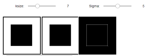
lena.jpg(ksize=7, sigma=5)

Canny 에지 검출

위에서 HPF인 미분 필터(Sobel, Laplacian)를 통하여 Feature의 특징을 알아보는 과정을 거쳤다.
이러한 Sobel, Laplacian과 같은 단순 이진 Filter를 사용하게 되면 크게 2가지의 단점이 발생하게 된다.
1. 검출한 Edge가 필요 이상으로 두꺼워 객체를 훨씬 더 식별 하기 어렵게 만든다.
2. 영상의 모든 중요한 Edge를 검출하기 위한 명확한 경계값을 찾기란 불가능할 때가 있다.(zero crossing을 통하여 특정 값 이상의 값을 찾는 것은 가능하다.)
이러한 2가지의 주된 문제점을 해결하기 위한 Algorithm이 Canny Algorithm이다.

Canny Algorithm
1. 가우시안 필터링을하여 영상을 부드럽게 한다.
2. Sobel 연산자를 사용하여 기울기(gradient)벡터의 크기(magnitude)를 계산
3. 가느다란 에지를 얻기 위해 3 x 3 창을 사용하여 gradient 벡터 방향에서 gradient 크기가 최대값인 화소만 남기고 나머지는 0으로 억제
위의 단계를 이해하기 위해서는 먼저 gradient 방향을 이해해야 한다.
예시를 살펴보기 위하여 $y=x^2$을 생각하면 다음과 같다.

사진 출처:sdolnote 블로그
위에 그래프에서 파란색 화살표를 보게 되면 Gradient 방향을 쉽게 알 수 있다.
x=-1 에서 x가 작아지는 방향을 가르키고 있다.(기울기가 음수)
x=1 에서 x가 커지는 방향을 가르키고 있다.(기울기가 양수)
위의 결과를 일반화 하여 생각하면 다음과 같다.
Gradient Descent가 가르키는 방향은 함수값이 커지는 방향이다.
위에서 사용한 도형을 생각하면 아래와 같은 결과를 얻을 수 있다.(흰색은 255, 검은색은 0값을 가진다.)

이러한 Gradient Descent의 방향은 Edge와 수직인 관계다.

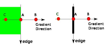
사진 출처:samsjang 블로그
위의 사진을 보게 되면 A지점에서 gradient값이 B,C보다 값이 큰지 아닌지를 체크한다.
A에서의 값이 가장 크면 그냥 다음단계로 넘어가고 그렇지 않으면 값을 0으로 만든다.

4. 연결된 에지를 얻기 위해 두 개의 임계값을 사용. 높은 값의 임계값을 사용하여 gradient 방향에서 낮은 값의 임계값이 나올 때까지 추적하며 에지를 연결하는 히스테리시스 임계값(hysteresis thresholig) 방식 사용

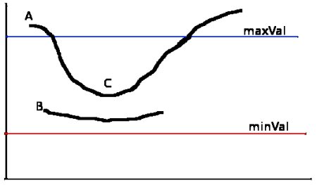
사진 출처:samsjang 블로그

A: maxVal보다 값이 크므로 Edge로 판단
B: minVal ~ maxVal사이에 있으나 A와 연결되지 않았으므로 제거
C: minVal ~ maxVal사이에 있으나 A와 연결되어 있으므로 남김
minVal보다 낮은값은 무조건 제거

#Component 선언
IntSlider_Threshold1 = IntSlider(
    value=0,
    min=0,
    max=300,
    step=1,
    description='threshold1: ',
    disabled=False,
    continuous_update=False,
    orientation='horizontal',
    readout=True,
    readout_format='d'
)

IntSlider_Threshold2 = IntSlider(
    value=0,
    min=0,
    max=300,
    step=1,
    description='threshold2: ',
    disabled=False,
    continuous_update=False,
    orientation='horizontal',
    readout=True,
    readout_format='d'
)

def layout(header, left, right):
    layout = AppLayout(header=header,
          left_sidebar=left,
          center=None,
          right_sidebar=right)
    return layout

wImg_original = Image(layout = Layout(border="solid"), width="50%")
wImg_Canny = Image(layout = Layout(border="solid"), width="50%")

items = [IntSlider_Threshold1,IntSlider_Threshold2]
Trick_Bar = Box(items)
box = layout(Trick_Bar,wImg_original,wImg_Canny)


tab_nest = widgets.Tab()
tab_nest.children = [box]
tab_nest.set_title(0, 'Canny 에지검출')
tab_nest

img = cv2.imread('./data/lena.jpg',0)
tmpStream = cv2.imencode(".jpeg", img)[1].tostring()
wImg_original.value = tmpStream

display.display(tab_nest)

#Event 선언
threshold1, threshold2 = 0,0
    

def on_value_change_Threshold1(change):
    global threshold1, threshold2
    threshold1 = change['new']
    Canny_img = cv2.Canny(img,threshold1, threshold2)
    tmpStream = cv2.imencode(".jpeg", Canny_img)[1].tostring()
    wImg_Canny.value = tmpStream
   
    
def on_value_change_Threshold2(change):
    global threshold1, threshold2
    threshold2 = change['new']
    Canny_img = cv2.Canny(img,threshold1, threshold2)
    tmpStream = cv2.imencode(".jpeg", Canny_img)[1].tostring()
    wImg_Canny.value = tmpStream

#초기화 작업
Canny_img = cv2.Canny(img,threshold1, threshold2)
tmpStream = cv2.imencode(".jpeg", Canny_img)[1].tostring()
wImg_Canny.value = tmpStream

#Component에 Event 장착
IntSlider_Threshold1.observe(on_value_change_Threshold1, names='value')
IntSlider_Threshold2.observe(on_value_change_Threshold2, names='value')

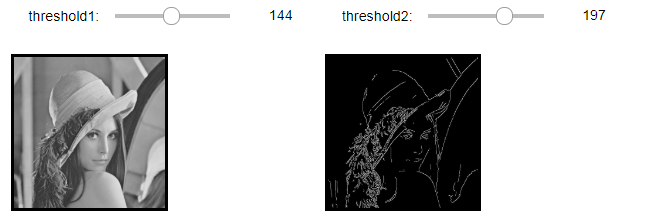
Canny 에지 검출 결과(threshold1=144, threshold2=197)

일반적인 필터 연산

cv2.filter2D(src, ddepth, kernel[, dst[, anchor[, delta[, borderType]]]]): Kernel을 통하여 Image를 Filtering하는 방법

cv2.sepFilter2D(src, ddepth, kernelX, kernelY[, dst[, anchor[, delta[, borderType]]]]): image의 x, y를 각각의 kernel을 통하여 Filtering하는 방법
parameter

kenelX: image x-축에 적용할 kernel
kenelY: image y-축에 적용할 kernel

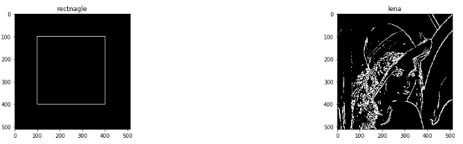
cv2.filter2D()와 cv2.sepFilter2D()에 의한 에지 검출

현재 Image를 Filtering하는 Filter를 Sobel Filter를 사용하여 1차미분 기반으로하는 Edge검출을 하였다.

src1 = cv2.imread('./data/rectangle.jpg',0)
src2 = cv2.imread('./data/lena.jpg',0)

kx,ky = cv2.getDerivKernels(1,0,ksize=3)
sobelX = ky.dot(kx.T)
print('kx=',kx)
print('ky=',ky)
print('sobelX=',sobelX)
gx = cv2.filter2D(src1,cv2.CV_32F,sobelX)
gx2 = cv2.sepFilter2D(src2,cv2.CV_32F,kx,ky)

kx,ky = cv2.getDerivKernels(0,1,ksize=3)
sobelY = ky.dot(kx.T)
print('kx=',kx)
print('ky=',ky)
print('sobelY=',sobelY)
gy = cv2.filter2D(src1,cv2.CV_32F,sobelY)
gy2 = cv2.sepFilter2D(src2,cv2.CV_32F,kx,ky)

mag = cv2.magnitude(gx,gy)
ret,edge = cv2.threshold(mag,100,255,cv2.THRESH_BINARY)

mag2 = cv2.magnitude(gx2,gy2)
ret2,edge2 = cv2.threshold(mag2,100,255,cv2.THRESH_BINARY)

plt.figure(figsize=(20,4))
imgae1=plt.subplot(1,2,1)
imgae1.set_title('rectnagle')
plt.imshow(edge, cmap="gray")

imgae2=plt.subplot(1,2,2)
imgae2.set_title('lena')
plt.imshow(edge2, cmap="gray")

plt.show()

cv2.filter2D()와 cv2.sepFilter2D()에 의한 에지 검출 결과

kx= [[-1.]
 [ 0.]
 [ 1.]]
ky= [[1.]
 [2.]
 [1.]]
sobelX= [[-1.  0.  1.]
 [-2.  0.  2.]
 [-1.  0.  1.]]
kx= [[1.]
 [2.]
 [1.]]
ky= [[-1.]
 [ 0.]
 [ 1.]]
sobelY= [[-1. -2. -1.]
 [ 0.  0.  0.]
 [ 1.  2.  1.]]

Log필터링, 0-교차 에지 영상

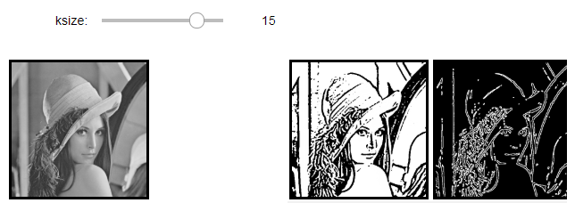
Log(Laplacian of Gaussian)을 위에서 Laplacian 필터링이 잡음에 민감하다는 특징때문에 위에서 작업하였던 Gausian Filter를 통하여 Noise제거후 Laplacian Filter를 적용시키는 방법이다.
2개의 Filter를 적용하는 것이아니라 하나의 Filter로서 선언하여 빠르게 결과를 얻을 수 있다.

또한 zerocrossing을 통하여 임계값 이상의 값만 출력하였다.

LoG Filter 식

$$LoG(x,y) = -\frac{1}{\pi \sigma^4}[1-\frac{x^2+y^2}{2\sigma^2}]exp(-\frac{x^2+y^2}{2\sigma^2})$$

#Component 선언
IntSlider_Ksize = IntSlider(
    value=1,
    min=1,
    max=20,
    step=2,
    description='ksize: ',
    disabled=False,
    continuous_update=False,
    orientation='horizontal',
    readout=True,
    readout_format='d'
)


def layout(header, left, right):
    layout = AppLayout(header=header,
          left_sidebar=left,
          center=None,
          right_sidebar=right)
    return layout

wImg_original = Image(layout = Layout(border="solid"), width="50%")
wImg_LoG = Image(layout = Layout(border="solid"), width="50%")
wImg_ZeroCrossing = Image(layout = Layout(border="solid"), width="50%") 

items = [wImg_LoG,wImg_ZeroCrossing]
Output = Box(items)
box = layout(IntSlider_Ksize,wImg_original,Output)

tab_nest = widgets.Tab()
tab_nest.children = [box]
tab_nest.set_title(0, 'Zero Crossing')
tab_nest

img = cv2.imread('./data/lena.jpg',0)
tmpStream = cv2.imencode(".jpeg", img)[1].tostring()
wImg_original.value = tmpStream

display.display(tab_nest)

#Event 선언
ksize, sigma = 1,0

def on_value_change_Ksize(change):
    global ksize, sigma
    ksize = change['new']
    
    kernel = logFilter()
    LoG = cv2.filter2D(img,cv2.CV_32F,kernel)
    LoG_img = LoG.astype(np.uint8)
    
    tmpStream = cv2.imencode(".jpeg", LoG_img)[1].tostring()
    wImg_LoG.value = tmpStream
    
    edgeZ = zeroCrossing(LoG)
    tmpStream = cv2.imencode(".jpeg", edgeZ)[1].tostring()
    wImg_ZeroCrossing.value = tmpStream
    
    
    
def logFilter():
    global ksize
    k2 = ksize//2
    sigma = 0.3 * (k2-1)+0.8
    print('sigma=',sigma)
    LoG = np.zeros((ksize,ksize),dtype=np.float32)
    for y in range(-k2,k2+1):
        for x in range(-k2,k2+1):
            g = -(x*x+y*y)/(2.0*sigma**2.0)
            LoG[y+k2,x+k2] = -(1.0+g)*np.exp(g)/(np.pi*sigma**4.0)
    return LoG        


def zeroCrossing(lap,thresh=0.01):
    width,height = lap.shape
    Z = np.zeros(lap.shape,dtype=np.uint8)
    for y in range(1,height-1):
        for x in range(1,width-1):
            neighbors = [lap[y-1,x],lap[y+1,x],lap[y,x-1],lap[y,x+1],
            lap[y-1,x-1],lap[y-1,x+1],
            lap[y+1,x-1],lap[y+1,x+1]]
            pos = 0
            neg = 0
            for value in neighbors:
                if value>thresh:
                    pos+=1
                if value<thresh:
                    neg+=1
            if pos > 0 and neg > 0:
                Z[y,x] = 255
    
    return Z
           

#초기화 작업
kernel = logFilter()
LoG = cv2.filter2D(img,cv2.CV_32F,kernel)
LoG_img = LoG.astype(np.uint8)

tmpStream = cv2.imencode(".jpeg", LoG_img)[1].tostring()
wImg_LoG.value = tmpStream
    
edgeZ = zeroCrossing(LoG)
tmpStream = cv2.imencode(".jpeg", edgeZ)[1].tostring()
wImg_ZeroCrossing.value = tmpStream


#Component에 Event 장착
IntSlider_Ksize.observe(on_value_change_Ksize, names='value')

Log필터링, 0-교차 에지 영상 결과(ksize=15)

모폴리지 연산

모폴리지 연산(morphological operation)은 구조 요소(structuring element)를 이용하여 반복적으로 영역을 확장시켜 떨어진 부분 또는 구멍을 채우거나, 잡음을 축소하여 제거하는 등의 연산으로 침식(Erosion), 팽창(dilate), 열기(opening), 닫기(closing)등 이 있다.

Erosion
해당 픽셀에서 structuring element를 범위안에서 극소값을 찾는 반환한다.
그레이 스케일 영상에서는 반복적인 min 필터링과 같다.
cv2.erode(img, kenel, iterations=1)
parameter

img: Erosion을 수행할 원본 이미지
kernel: Erosion을 위한 Kernel
iterations: Erosion 반복 횟수

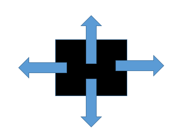
Dilation
해당 픽셀에서 structuring element를 범위안에서 극대값을 찾는 반환한다.
그레이 스케일 영상에서는 반복적인 max 필터링과 같다.
cv2.dilate(img, kenel, iterations=1)
parameter

img: Dilation 수행할 원본 이미지
kernel: Dilation 위한 Kernel
iterations: Erosion 반복 횟수

모폴로지 연산
모폴로지 op연산을 iterations만큼 반복한다.
cv2.morphologyEx(img, op, kenel, iterations=1)

morphology op

op	설명
cv2.MORPH_OPEN	dst = dilate(erode(src,kernel),kernel)
cv2.MORPH_Close	dst = erode(dilate(src,kernel),kernel)
cv2.MORPH_GRADIENT	dst = dilate(src,kernel)-erode(src,kernel)
cv2.MORPH_TOPHAT	dst = src - open(src,kernel)
cv2.MORPH_BLACKHAT	dst = close(src,kernel) - src

Structuring Element
특정 모양의 structuring element를 만들어서 적용할 수 있다.
cv2.getStructuringElement(shape, ksize[, anchor])
parameter

shape: Element의 모양
MORPH_RECT: 사각형
MORPH_CROSS: 십자 모양
MORPH_ELLIPSE: 타원형 모양
ksize: structuring element 사이즈

모폴리지 연산1

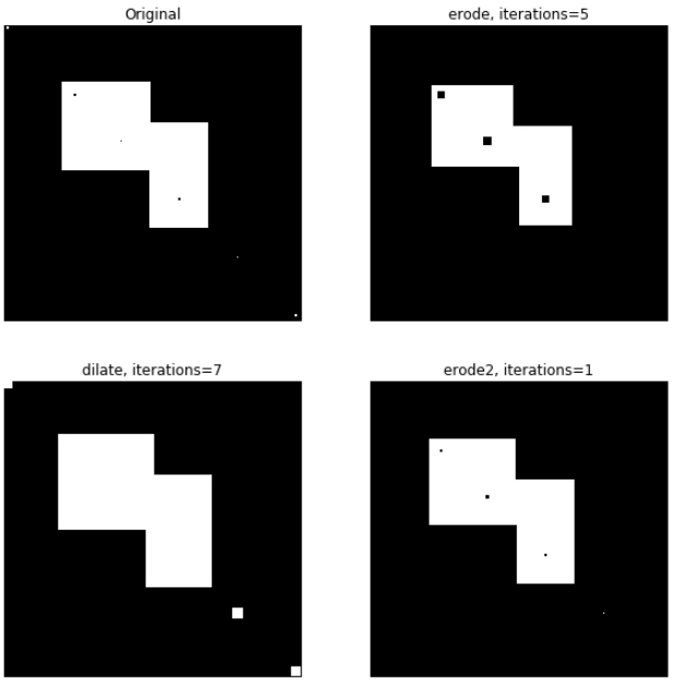
erode: 연산결과 최소값 pixel인 검은색(0)이 점점커지거나 흰색이 제거되는것을 확인할 수 있다.
dilate: 연산결과 최재값 pixel인 흰색(255)이 점점커지거나 검은색이 제거되는것을 확인할 수 있다.

src = cv2.imread('./data/morphology.jpg',0)
kernel = cv2.getStructuringElement(shape=cv2.MORPH_RECT,ksize=(3,3))
erode = cv2.erode(src,kernel,iterations=5)
dilate = cv2.dilate(src,kernel,iterations=7)
erode2 = cv2.erode(src,kernel,iterations=1)

plt.figure(figsize=(10,10))
imgae1=plt.subplot(2,2,1)
imgae1.set_title('Original')
plt.axis('off')
plt.imshow(src, cmap="gray")

imgae2=plt.subplot(2,2,2)
imgae2.set_title('erode, iterations=5')
plt.axis('off')
plt.imshow(erode, cmap="gray")

imgae3=plt.subplot(2,2,3)
imgae3.set_title('dilate, iterations=7')
plt.axis('off')
plt.imshow(dilate, cmap="gray")

imgae4=plt.subplot(2,2,4)
imgae4.set_title('erode2, iterations=1')
plt.axis('off')
plt.imshow(erode2, cmap="gray")

plt.show()

모폴리지 연산1 결과

morphologyEx()

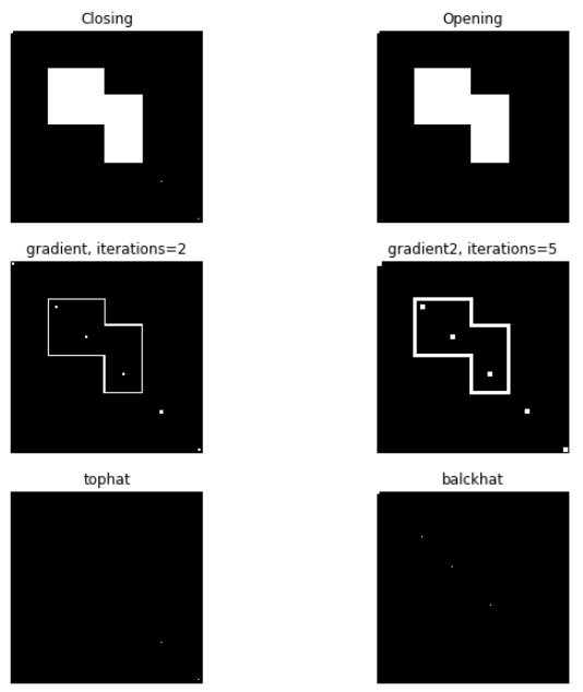
opening: erode 후 dilate를 연산, 검은물체 내에 흰색 잡음 제거
closing: dilate 후 erode연산, 흰색 물체 속의 검은색 잡음 제거
gradient: dilate - erode, 최대값 - 최소값으로서 급격한 차이를 가지는 Edge추출

src = cv2.imread('./data/morphology.jpg',0)
kernel = cv2.getStructuringElement(shape=cv2.MORPH_RECT,ksize=(3,3))
closing = cv2.morphologyEx(src,cv2.MORPH_CLOSE,kernel,iterations=5)
opening = cv2.morphologyEx(closing,cv2.MORPH_OPEN,kernel,iterations=5)
gradient = cv2.morphologyEx(src,cv2.MORPH_GRADIENT,kernel,iterations=2)
gradient2 = cv2.morphologyEx(src,cv2.MORPH_GRADIENT,kernel,iterations=5)

tophat= cv2.morphologyEx(src,cv2.MORPH_TOPHAT,kernel,iterations=5)
balckhat= cv2.morphologyEx(src,cv2.MORPH_BLACKHAT,kernel,iterations=5)

plt.figure(figsize=(10,10))
imgae1=plt.subplot(3,2,1)
imgae1.set_title('Closing')
plt.axis('off')
plt.imshow(closing, cmap="gray")

imgae2=plt.subplot(3,2,2)
imgae2.set_title('Opening')
plt.axis('off')
plt.imshow(opening, cmap="gray")

imgae3=plt.subplot(3,2,3)
imgae3.set_title('gradient, iterations=2')
plt.axis('off')
plt.imshow(gradient, cmap="gray")

imgae4=plt.subplot(3,2,4)
imgae4.set_title('gradient2, iterations=5')
plt.axis('off')
plt.imshow(gradient2, cmap="gray")

imgae5=plt.subplot(3,2,5)
imgae5.set_title('tophat')
plt.axis('off')
plt.imshow(tophat, cmap="gray")

imgae6=plt.subplot(3,2,6)
imgae6.set_title('balckhat')
plt.axis('off')
plt.imshow(balckhat, cmap="gray")

plt.show()

morphologyEx() 결과

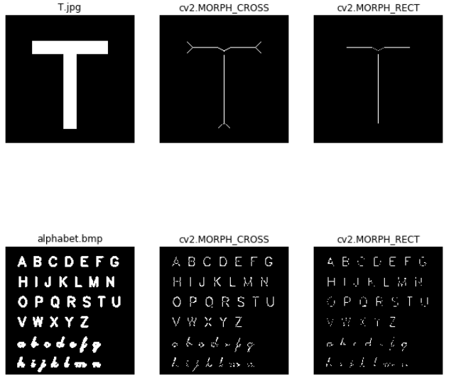
모폴로지 연산 골격화

각각의 T, alphabet에 십자모양, 사각형 모양의 structuring element를 생성 뒤 모폴리지 open 적용

src = cv2.imread('./data/T.jpg',0)
src2 = cv2.imread('./data/alphabet.bmp',0)

ret,A = cv2.threshold(src,128,255,cv2.THRESH_BINARY)
ret,B = cv2.threshold(src2,128,255,cv2.THRESH_BINARY)

shape1 = cv2.MORPH_CROSS
shape2 = cv2.MORPH_RECT

C = cv2.getStructuringElement(shape=shape1,ksize=(7,7))
D = cv2.getStructuringElement(shape=shape2,ksize=(7,7))

def skel_func(img,option=0):
    done = True
    A_1 = img
    A_2 = img
    skel_dst = np.zeros(src.shape,np.uint8)
    skel_dst2 = np.zeros(src.shape,np.uint8)

    while done:
        erode = cv2.erode(A_1,C)
        
        opening = cv2.morphologyEx(erode,cv2.MORPH_OPEN,C)
        
            
        tmp = cv2.subtract(erode,opening)
        
        erode2 = cv2.erode(A_2,D)
        opening2 = cv2.morphologyEx(erode,cv2.MORPH_OPEN,D)
        tmp2 = cv2.subtract(erode2,opening2)
        
        skel_dst = cv2.bitwise_or(skel_dst,tmp)
        skel_dst2 = cv2.bitwise_or(skel_dst2,tmp2)
        
        A_1 = erode.copy()
        A_2 = erode.copy()
        
        done = (cv2.countNonZero(A_1) !=0) and (cv2.countNonZero(A_2) !=0)
    return skel_dst,skel_dst2
    

skel_dst,skel_dst2 = skel_func(A)
skel_dst3,skel_dst4 = skel_func(B,1)

plt.figure(figsize=(10,10))

imgae1=plt.subplot(2,3,1)
imgae1.set_title('T.jpg')
plt.axis('off')
plt.imshow(src, cmap="gray")

imgae2=plt.subplot(2,3,2)
imgae2.set_title('cv2.MORPH_CROSS')
plt.axis('off')
plt.imshow(skel_dst, cmap="gray")

imgae2=plt.subplot(2,3,3)
imgae2.set_title('cv2.MORPH_RECT')
plt.axis('off')
plt.imshow(skel_dst2, cmap="gray")

imgae1=plt.subplot(2,3,4)
imgae1.set_title('alphabet.bmp')
plt.axis('off')
plt.imshow(src2, cmap="gray")

imgae2=plt.subplot(2,3,5)
imgae2.set_title('cv2.MORPH_CROSS')
plt.axis('off')
plt.imshow(skel_dst3, cmap="gray")

imgae2=plt.subplot(2,3,6)
imgae2.set_title('cv2.MORPH_RECT')
plt.axis('off')
plt.imshow(skel_dst4, cmap="gray")

plt.show()

모폴로지 연산 골격화 결과

템플릿 매칭

cv2.matchTemplate(image, templ, method[,result): 각 픽셀을 이동하면서 매칭 위치를 탐색하는 방법이다. 템플릿 매칭은 이동문제는 해결할 수 있지만, 회전 및 스케일링된 물체에 대한 매칭은 템플릿을 회전 및 스케일리시켜가며 여러 개의 템플릿을 이용할 수 있으나 어려운 문제이다.
템플릿 매칭에서 영상의 밝기를 그대로 사용할 수도 있고, 에지, 코너점, 주파수 변환 등의 특징 공간으로 변환하여 템플릿 매칭을 수행할 수 있으며, 영상의 밝기 등에 덜 민감하도록 정규화 과정이 필요하다.

parameter

image: 매칭 받을 이미지
templ: 매칭할 이미지
method: 매칭 방법

method

cv2.TM_SQDIFF: 템플릿 T를 탐색영역 I에서 이동시켜가며 차이의 제곱합계를 계산
cv2.TM_SQDIFF_NORMED: cv2.TM_SQDIFF를 정규화
cv2.TM_CCORR: 템플릿 T를 탐색영역 I에서 이동시켜가며 곱의 합계를 계산
cv2.TM_CCORR_NORMED: cv2.TM_CCORR를 정규화

src = cv2.imread('./data/alphabet.bmp',0)
src = cv2.bitwise_not(src)

tmp_A = cv2.imread('./data/A.bmp',0)
tmp_S = cv2.imread('./data/S.bmp',0)
tmp_b = cv2.imread('./data/b.bmp',0)
tmp_f_90 = cv2.imread('./data/f_90.bmp',0)

tmp_A = cv2.bitwise_not(tmp_A)
tmp_S = cv2.bitwise_not(tmp_S)
tmp_b = cv2.bitwise_not(tmp_b)
tmp_f_90 = cv2.bitwise_not(tmp_f_90)

dst = cv2.cvtColor(src,cv2.COLOR_GRAY2BGR)

font = cv2.FONT_HERSHEY_SIMPLEX

R1 = cv2.matchTemplate(src,tmp_A,cv2.TM_SQDIFF_NORMED)
minVal,_,minLoc,_ = cv2.minMaxLoc(R1)
print('TM_SQDIFF_NORMED: ',minVal, minLoc)

w,h = tmp_A.shape[:2]
cv2.rectangle(dst,minLoc,(minLoc[0]+h,minLoc[1]+w),(255,0,0),10)

text = 'Maching: A'
dx,dy = minLoc
dx = dx-10
dy = dy-10
org = (dx,dy)
cv2.putText(dst,text,org,font,1.3,(255,0,0),4)


R2 = cv2.matchTemplate(src,tmp_S,cv2.TM_SQDIFF_NORMED)
minVal,maxVal,minLoc,maxLoc = cv2.minMaxLoc(R2)

w,h = tmp_S.shape[:2]
cv2.rectangle(dst,minLoc,(minLoc[0]+h,minLoc[1]+w),(0,255,0),10)

text = 'Maching: S'
dx,dy = minLoc
dx = dx-10
dy = dy-10
org = (dx,dy)
cv2.putText(dst,text,org,font,1.3,(0,255,0),4)

R3 = cv2.matchTemplate(src,tmp_b,cv2.TM_SQDIFF_NORMED)
minVal,_,minLoc,_ = cv2.minMaxLoc(R3)

w,h = tmp_b.shape[:2]
cv2.rectangle(dst,minLoc,(minLoc[0]+h,minLoc[1]+w),(0,0,255),10)

text = 'Maching: b'
dx,dy = minLoc
dx = dx-10
dy = dy-10
org = (dx,dy)
cv2.putText(dst,text,org,font,1.3,(0,0,255),4)

R4 = cv2.matchTemplate(src,tmp_f_90,cv2.TM_SQDIFF_NORMED)
minVal,_,minLoc,_ = cv2.minMaxLoc(R4)

w,h = tmp_b.shape[:2]
cv2.rectangle(dst,minLoc,(minLoc[0]+h,minLoc[1]+w),(0,255,255),10)

text = 'Maching: f_90'
dx,dy = minLoc
dx = dx-120
dy = dy-10
org = (dx,dy)
cv2.putText(dst,text,org,font,1.3,(0,255,255),4)

plt.axis('off')
plt.imshow(dst)

템플릿 매칭 결과

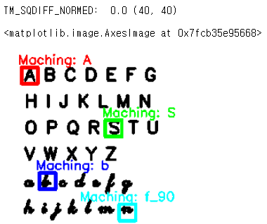
cv2에서 지원하는 템플렛 매칭의 경우 회전이나 글자크기는 Detect하지 못하는 한계점이 분명하게 존재한다.
결과를 확인하면 f를 회전한 alphabet은 잘못된 글자를 mapping하는 것을 확인할 수 있다.

참조:원본코드
참조:Python으로 배우는 OpenCV 프로그래밍
문제가 있거나 궁금한 점이 있으면 wjddyd66@naver.com으로 Mail을 남겨주세요.

Share on

Twitter Facebook LinkedIn

JeongYong Hwang