
OpenCV-영상 분할
참고사항
현재 Post에서 사용하는 Data를 만드는 법이나 사용한 Image는 github에 올려두었습니다.
영상 분할
영상 분할(image segmentation)은 입력 영상에서 관심 있는 영역을 분리하는 과정이다.
이러한 영상 분할은 영상 분석, 물체 인식, 추적 등 대부분의 영상처리 응용에서 필수적인 단계이다.
영상 분할은 크게 경계선 또는 영역으로 분할한다.
임계법 사용방법은 가장 간단한 영상 분할 방법으로 cv2.threshold(), cv2.adaptiveThreshold()로서 선수 과정으로 알고있어야 하는 지식이다.
사전 지식: 임계값과 히스토그램 처리
Hough 변환에 의한 직선, 원 검출
사전지식(극좌표)
Hough변환을 이해하기 위해서 Hough변환에 기초인 극좌표계를 이해해야한다.

사진 출처:위키피디아
위와 같은 직선이 존재할 때 일반적인 직선은 다음과 같이 표현될 수 있다.
$$y=mx$$
위와 같은 직선을 r((0,0) ~ (x,y)까지의 거리),\(\theta\)(각도)로서 표현하는 것이 극좌표 계이다.
아래 식으로서 극좌표계로 표현하는 식을 알아보자.
$$sin(\theta) = \frac{y}{r}, cos(\theta) = \frac{x}{r}$$
$$r^2 = x^2 + y^2$$
$$r^2 = xcos(\theta)r + ysin(\theta)r$$
$$r = xcos(\theta) + ysin(\theta)$$
위와 같은 식으로서 r,\(\theta\)로서 표현하게 되면 한 점(x,y)를 지나는 모든 직선을 구할수 있다.
Hough 변환
Hough변환은 (x,y)좌표공간의 픽셀들을 (r,\(\theta\))매개변수 공간에서 곡선의 형태로 나타난다.
또한 (x,y)좌표공간에서 같은 직선상에 존재하는 픽셀들의 경우 (r,\(\theta\))매개변수 공간에서 교점을 가지게 된다.
Hough변환 기법은 이러한 특징을 이용하여 영상의 특징 픽셀들을 (x,y)좌표 공간에서 (r,\(\theta\))의 극좌표로 나타내어 mapping 시킨 후 보팅 과정을 통해 교점을 찾아 직선 성분을 추출하는 기법이다.
위의 Hough변환의 설명으로는 이해하기 힘드므로 아래 사진을 참조하자.
아래 사진은 일직선상에있는 3개의 점에 대하여 극좌표를 시각적으로 나타낸 사진이다.
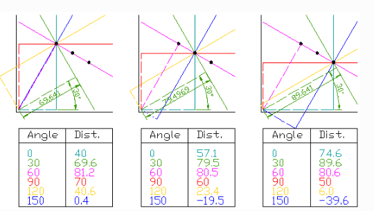
사진 출처:gramman 블로그
위의 사진의 결과를 아래처럼 (r,\(\theta\))에서 mapping하게되면 sin 그래프로서 나타낼 수 있는 것을 알 수 있다.
$$asinx + bcosx = \sqrt{a^2+b^2}sin(x+\theta)$$
$$sin(\theta) = \frac{b}{\sqrt{a^2+b^2}}, cos(\theta) = \frac{a}{\sqrt{a^2+b^2}}$$
위의 과정으로 sin형태로 그래프가 나온다는 것을 예상할 수 있고 실제로 그려보면 아래 사진과 같이 출력되게 된다.
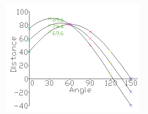
사진 출처:gramman 블로그
위와같이 곡선에서 중요하게 생각해야 하는것은 교점이 생겼다는 것 이다.
그래프에서 교점이 생겼다는 것은 다음과 같이 생각할 수 있다.
예를들어 다음과 같은 직선 2개가 존재한다고 생각하자.
$$r_1 = x_1cos(\theta_1) + y_1sin(\theta_1)$$
$$r_2 = x_2cos(\theta_2) + y_2sin(\theta_2)$$
두개의 곡선을 극좌표계로 Mapping하였을때의 교점은 (\((x_1,y_1)\))을 지나는 직선들중 하나의 직선과 (\((x_2,y_2)\))지나는 직선들 중 하나의 직선이 같아졌다는 것을 의미한다.
즉, (\((x_1,y_1)\))과 (\((x_2,y_2)\))는 하나의 같은 점선 위에 있다는 것을 알 수 있다.
이러한 방식을 통하여 Hough 변환은 교점을 찾아 직선 성분을 추출할 수 있다.
이러한 직선은 Edge, blur와 같이 Image에서 주요한 Feature로서 사용될 수 있기 때문에 주요한 특성이다.
참조:iskim3068 블로그
OpenCV를 통한 Hough변환
cv2.HoughLines(image, rho, theta, threshold[, lines[, srn[, stn[, min_theta[, max_theta]]]]]): Hough변환을 통하여 직선을 검출
parameter
- image: input(canny edge선 적용 후)
- rho: r값의 범위(0~1 실수)
- theata: \(\theta\)값의 범위(0~180 정수)
- threshold: 만나는 점의 기준, 숫자가 적으면 많은 선이 검출되지만 정확도가 떨어지고, 숫자가 크면 정확도가 올라감
cv2.HoughLinesP(image, rho, theta, threshold, minLineLength, maxLineGap): cv2.HoughLines는 모든 점에 대해서 계산하므로 시간이 오래걸린다. 따라서 모든 점을 대상으로 하는 것이 아니라 임의의 점을 이용하여 직선을 찾는 방법이다. 단, 임계값을 작게 하여야 한다.
선의 시작점과 끝점을 Return해주기 때문에 쉽게 화면에 표현할 수 있다.
parameter
- image: input(canny edge선 적용 후)
- rho: r값의 범위(0~1 실수)
- theata: \(\theta\)값의 범위(0~180 정수)
- threshold: 만나는 점의 기준, 숫자가 적으면 많은 선이 검출되지만 정확도가 떨어지고, 숫자가 크면 정확도가 올라감
- minLineLength: 선의 최소 길이
- maxLineGap: 선과 선사이의 최대 허용간격
cv2.HoughCircles(image, method, dp, minDist[, circles[, param1[, param2[, minRadius[, maxRadius]]]]])
$$(x-x_{center})^2 + (y-y_{center})^2 = r^2$$
3개의 변수에 대하여 계산하는 것은 비효율적이므로 가장자리에서 기울기를 측정하여 원을 그리는데 관련이 있는 점인지를 확인할 수 있는 Hough Gradient Method를 사용
parameter
- image: input(canny edge선 적용 후)
- method: 검출방법, ex)HOUGH_GRADIENT
- dp: 해상도
- minDist: 검출한 원의 중심과의 최소거리. 값이 작으면 원이 아닌 것들도 검출이 되고, 너무 크면 원을 놓칠 수 있음
- param1: 내부적으로 사용하는 canny edge 검출기에 전달되는 Paramter
- param2: 이 값이 작을 수록 오류가 높아짐. 크면 검출률이 낮아짐.
- minRadius: 원의 최소 반지름.
- maxRadius: 원의 최대 반지름.
참고사항(Hough Circle Transform): navisphere 블로그
직선검출: cv2.HoughLines(), cv2.HoughLinesP()
1
2
3
4
5
6
7
8
9
10
11
12
13
14
15
16
17
18
19
20
21
22
23
24
25
26
27
28
29
30
31
32
33
34
35
36
37
38
39
40
41
42
43
44
45
46
47
48
49
50
51
52
53
54
def layout(header, left, right):
    layout = AppLayout(header=header,
          left_sidebar=left,
          center=None,
          right_sidebar=right)
    return layout

wImg_original = Image(layout = Layout(border="solid"), width="20%")
wImg_Edges = Image(layout = Layout(border="solid"), width="20%")
wImg_Lines = Image(layout = Layout(border="solid"), width="20%")
wImg_Lines2 = Image(layout = Layout(border="solid"), width="20%")

items = [wImg_original,wImg_Edges,wImg_Lines,wImg_Lines2]
wImg=Box(items)

display.display(wImg)

src = cv2.imread('./data/rectangle.jpg')
src2 = src.copy()
gray = cv2.cvtColor(src,cv2.COLOR_BGR2GRAY)
edges = cv2.Canny(src,0,200)
lines = cv2.HoughLines(edges,rho=1,theta=np.pi/180.0,threshold=100)
lines2 = cv2.HoughLinesP(edges,rho=1,theta=np.pi/180.0,threshold=100)

print('HoughLines lines.shape=',lines.shape)
print('HoughLinesP lines.shape=',lines2.shape)

for line in lines:
    rho,theta = line[0]
    c = np.cos(theta)
    s = np.sin(theta)
    x0 = c*rho
    y0 = s*rho
    x1 = int(x0+1000*(s))
    y1 = int(y0+1000*(c))
    x2 = int(x0-1000*(s))
    y2 = int(y0-1000*(c))
    cv2.line(src,(x1,y1),(x2,y2),(0,0,255),2)

tmpStream = cv2.imencode(".jpeg", gray)[1].tostring()
wImg_original.value = tmpStream

tmpStream = cv2.imencode(".jpeg", edges)[1].tostring()
wImg_Edges.value = tmpStream

tmpStream = cv2.imencode(".jpeg", src)[1].tostring()
wImg_Lines.value = tmpStream

for line in lines2:
    x1,y1,x2,y2 = line[0]
    cv2.line(src2,(x1,y1),(x2,y2),(0,0,255),10)

tmpStream = cv2.imencode(".jpeg", src2)[1].tostring()
wImg_Lines2.value = tmpStream
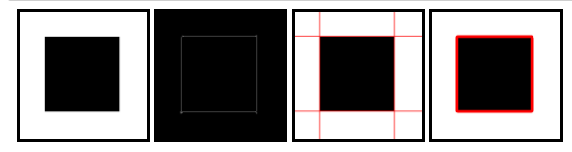
직선검출: cv2.HoughLines(), cv2.HoughLinesP() 결과
HoughLines lines.shape= (4, 1, 2)
HoughLinesP lines.shape= (4, 1, 4)
원 검출: cv2.HoughCircles()
1
2
3
4
5
6
7
8
9
10
11
12
13
14
15
16
17
18
19
20
21
22
23
24
25
26
27
28
src1 = cv2.imread('./data/circle.jpg')
gray1 = cv2.cvtColor(src1,cv2.COLOR_BGR2GRAY)
circle1 = cv2.HoughCircles(gray1,method=cv2.HOUGH_GRADIENT,dp=1,minDist=50,param2=15,minRadius=40,maxRadius=100)
print('circle1.shape= ',circle1.shape)
for circle in circle1[0,:]:
    cx,cy,r = circle
    cv2.circle(src1,(cx,cy),r,(0,0,255),2)

src2 = cv2.imread('./data/circle2.jpg')
gray2 = cv2.cvtColor(src2,cv2.COLOR_BGR2GRAY)
circle2 = cv2.HoughCircles(gray2,method=cv2.HOUGH_GRADIENT,dp=1,minDist=50,param2=15)
print('circle2.shape= ',circle2.shape)
for circle in circle2[0,:]:
    cx,cy,r = circle
    cv2.circle(src2,(cx,cy),r,(0,0,255),10)

plt.figure(figsize=(20,4))
imgae1=plt.subplot(1,2,1)
imgae1.set_title('circles.jpg')
plt.axis('off')
plt.imshow(src1, cmap="gray")

imgae2=plt.subplot(1,2,2)
imgae2.set_title('circles2.jpg')
plt.axis('off')
plt.imshow(src2, cmap="gray")

plt.show()
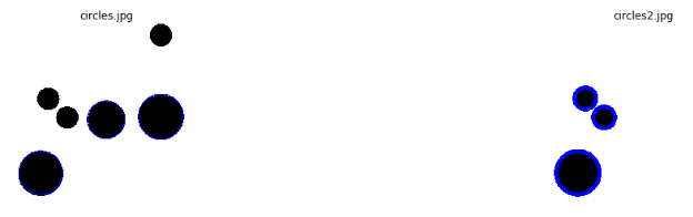
원 검출: cv2.HoughCircles() 결과
circle1.shape= (1, 3, 3)
circle2.shape= (1, 3, 3)
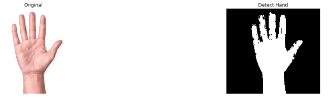
컬러 범위에 의한 영역 분할
cv2.inRange(src,lowerb,upperb[,dst]): loweb ~ upperb 범위의 컬러 영역을 분할할 수 있다. Color -> HSV 색상으로 변환 후에, 색상 범위를 지정하여 손, 얼굴 등의 피부 검출등을 분할할 때 유용한다.
parameter
- src: input
- lowerb: 최소값
- upperb: 최대값
1
2
3
4
5
6
7
8
9
10
11
12
13
14
15
16
17
18
19
src = cv2.imread('./data/hand.jpg')
hsv = cv2.cvtColor(src,cv2.COLOR_BGR2HSV)
lower = (0,30,0)
upper = (150,200,255)
dst = cv2.inRange(hsv,lower,upper)

src = cv2.cvtColor(src,cv2.COLOR_BGR2RGB)
plt.figure(figsize=(20,4))
imgae1=plt.subplot(1,2,1)
imgae1.set_title('Original')
plt.axis('off')
plt.imshow(src)

imgae2=plt.subplot(1,2,2)
imgae2.set_title('Detect Hand')
plt.axis('off')
plt.imshow(dst, cmap="gray")

plt.show()
컬러 범위에 의한 영역 분할 결과
윤각선 검출 및 그리기
컨투어(contour)란 동일한 색 또는 동일한 픽셀값(강도, itensity)을 가지고 있는 영역의 경계선 정보이다.
cv2.findContours(image,mode,method[,contours[,hierarchy[,offset]]]): image의 countour를 반환한다.
parameter
- image: 흑백이미지 또는 이진화된 이미지
- mode: 컨투어를 찾는 방법
- cv2.RETR_EXTERNAL: 가장 외각의 윤각선만 찾는다
- cv2.RETR_LIST: 모든 윤각선을 찾는다. 계층관계를 설정하지 않는다.
- cv2.RETR_CCOMP: 2레벨 계층 구조로 모든 윤각선을 찾는다.
- cv2.RETR_TREE: 모든 윤각선을 계층적 트리 형태로 찾는다.
- method: 컨투어를 찾을 때 사용하는 근사화 방법
- cv2.CHAIN_APPROX_NONE: 체인 코드로 표현된 윤각선의 모든 좌표를 반환한다.
- cv2.CHAIN_APPROX_SIMPLE: 윤각선의 다각형 근사 좌표를 변환한다.
- cv2.CHAIN_APPROX_TC89_L1: Teh-Chin의 체인 코드 알고리즘으로 근사화 한다.
- cv2.CHAIN_APPROX_RC89_KCOS: 위와 같음
cv2.drawContours(image,contours,contourldx,color[,thickness[,lineType[,hierarcht[,maxLevel[,offset]]]]]): 컨투어 정보에서 비트맵 이미지 생성
parameter
- image: 원본 이미지
- contours: 컨투어 라인 정보
- contourldx: 컨투어 라인 번호
- color: 색상
참고사항
현재 Window와 Linux환경에서 번갈아가면서 작업하고 있다.
OpenCV의 version은 4.1.1로 동일하나 cv.findContours가 반환하는 인자의 개수가 다르다.
- Window: image,contours,hierarchy
- Linux: contours,hierarchy
함수 사용시 Error가 발생하게 되면 Return 인자의 개수를 변형해보는 것이 가장먼저 확인해야 하는 작업이다.
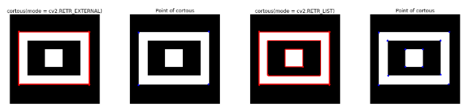
윤각선 검출 및 그리기
- mode: cv2.RETR_EXTERNAL, cv2.RETR_LIST
- method: cv2.CHAIN_APPROX_SIMPLE
현재 method로서 cv2.CHAIN_APPROX_SIMPLE을 사용하여 윤각선의 다각형 근사 좌표를 반환하도록 하였다.
이런 이유로 정확한 좌표의 위치가 아닌 원하는 좌표에서 -10 ~ +10차이의 오차를 보이는 많은 점이 반환되었다.
따라서 delete_duplicated_contours를 통하여 근사한 위치에 존재하는 점을 하나로 통일하는 과정을 거친 뒤 결과를 출력하였다.
1
2
3
4
5
6
7
8
9
10
11
12
13
14
15
16
17
18
19
20
21
22
23
24
25
26
27
28
29
30
31
32
33
34
35
36
37
38
39
40
41
42
43
44
45
46
47
48
49
50
51
52
53
54
55
56
57
58
59
60
61
62
63
64
65
66
67
68
69
70
71
72
73
src = cv2.imread('./data/rectangle2.jpg')
src2 = np.copy(src)
src3 = np.copy(src)
src4 = np.copy(src)

gray = cv2.cvtColor(src,cv2.COLOR_BGR2GRAY)

mode = cv2.RETR_EXTERNAL
mode2 = cv2.RETR_LIST
method = cv2.CHAIN_APPROX_SIMPLE

contours, hierachy = cv2.findContours(gray,mode,method)
contours2, hierachy2 = cv2.findContours(gray,mode2,method)

print('contours1')
print('type(contorous)=',type(contours))
print('type(contorous[0])=',type(contours[0]))
print('len(contours)=',len(contours))
print('contours[0].shape=',contours[0].shape)
print('contours[0]=',contours[0])
print('-'*20)
print('contours2')
print('type(contorous2)=',type(contours2))
print('type(contorous2[0])=',type(contours2[0]))
print('len(contours2)=',len(contours2))
print('contours2[0].shape=',contours2[0].shape)
print('contours2[0]=',contours2[0])

def delete_duplicated_contours(contours):
    pt_array=[]
    for c in contours:
        for pt in range(0,len(c)):
            b = True
            for pt_arr in pt_array:
                if((pt_arr[0]>c[pt][0][0] - 10 and c[pt][0][0] + 10 > pt_arr[0]) and (pt_arr[1]>c[pt][0][1] - 10 and c[pt][0][1] + 10 > pt_arr[1])):
                    b = False
            if(b):
                pt_array.append(c[pt][0])
    return pt_array

pt_array1=delete_duplicated_contours(contours)
pt_array2=delete_duplicated_contours(contours2)

cv2.drawContours(src,contours,-1,(255,0,0),3)
cv2.drawContours(src3,contours2,-1,(255,0,0),3)

for pt in pt_array1:
    cv2.circle(src2,(pt[0],pt[1]),5,(0,0,255),-1)

for pt in pt_array2:
    cv2.circle(src4,(pt[0],pt[1]),5,(0,0,255),-1)

plt.figure(figsize=(20,4))

imgae1=plt.subplot(1,4,1)
imgae1.set_title('cortous(mode = cv2.RETR_EXTERNAL)')
plt.axis('off')
plt.imshow(src)

imgae2=plt.subplot(1,4,2)
imgae2.set_title('Point of cortous')
plt.axis('off')
plt.imshow(src2)

imgae1=plt.subplot(1,4,3)
imgae1.set_title('cortous(mode = cv2.RETR_LIST)')
plt.axis('off')
plt.imshow(src3)

imgae2=plt.subplot(1,4,4)
imgae2.set_title('Point of cortous')
plt.axis('off')
plt.imshow(src4)
윤각선 검출 및 그리기
contours1
type(contorous)= <class 'list'>
type(contorous[0])= <class 'numpy.ndarray'>
len(contours)= 10
contours[0].shape= (1, 1, 2)
contours[0]= [[[ 48 405]]]
--------------------
contours2
type(contorous2)= <class 'list'>
type(contorous2[0])= <class 'numpy.ndarray'>
len(contours2)= 20
contours2[0].shape= (1, 1, 2)
contours2[0]= [[[ 48 405]]]
영역 채우기, 인페인트, 거리계산, 워터쉐드
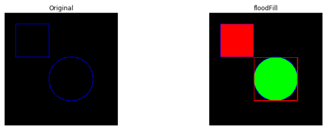
cv2.floodFill()영역 채우기
cv2.floodFill(image, mask, seedPoint, newVal[, loDiff[, upDiff[, flags]]]): Starting Point 으로부터 Edge까지 지정한 Pixel값 채우기
parameter
- image: Input
- mask: a single-channel 8-bit image, 2 pixels wider and 2 pixels taller than image.
- seedPoint: starting Point
- newVal: 안을 채울 새로운 Pixel 값
- loDiff: 현재 Pixel과의 차이의 최소값
- upDiff: 현재 Pixel과의 차이의 최대값
- flag
- Link4: 이웃한 4 픽셀을 고려한다.
- Link8: 이웃한 8픽셀을 고려한다.
- FixedRange: 시드 픽셀간의 차이를 고려한다.
- MaskOnly: 이미지를 변경하지 않고, 마스크를 채운다.
return
- mask: 지정한 조건으로 이미지를 채운값
- rect: mask의 바운딩 사각형
식
$$src(x^{\prime},y^{\prime}) - loDiff \leq src(x,y) \leq src(x^{\prime},y^{\prime}) + upDiff$$
1
2
3
4
5
6
7
8
9
10
11
12
13
14
15
16
17
18
19
20
21
22
23
24
25
26
27
src = np.zeros((512,512,3),dtype=np.uint8)

cv2.rectangle(src,(50,50),(200,200),(0,0,255),2)
cv2.circle(src,(300,300),100,(0,0,255),2)

dst = src.copy()
cv2.floodFill(dst,mask=None,seedPoint=(100,100),newVal=(255,0,0))

retval,dst2,mask,rect = cv2.floodFill(dst,mask=None,seedPoint=(300,300),newVal=(0,255,0))

print('rect=',rect)
x,y,width,height = rect
cv2.rectangle(dst2,(x,y),(x+width,y+height),(255,0,0),2)

plt.figure(figsize=(20,4))

imgae1=plt.subplot(1,3,1)
imgae1.set_title('Original')
plt.axis('off')
plt.imshow(src)

imgae2=plt.subplot(1,3,2)
imgae2.set_title('floodFill')
plt.axis('off')
plt.imshow(dst)

print(retval)
cv2.floodFill()영역 채우기 결과
rect= (202, 202, 197, 197)
30519
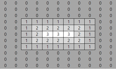
cv2.distancdTransform() 거리계산
cv2.distanceTransform(src, distanceType, maskSize[, dst]): 0이 아닌 화소에서 가장 가까운 0인 화소까지의 거리를 계산
parameter
- src: Input
- distanceType: 거리계산 방식
- CV_DIST_L1
- CV_DIST_L2
- CV_DIST_C
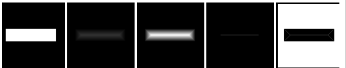
위의 cv2.distanceTransform()을 그림으로 살펴보면 아래와 같다.
사진 출처:webnautes 블로그
아래의 결과는 왼쪽순서대로 다음과 같다.

- src: 원본 사진
- dist:
cv2.distanceTransform()결과 - dst: dist를 Normalization을 통해 선명하게 출력
- dst2:
cv2.threshold()을 통하여 최대값만 출력 - dst3: dist의 edge출력 후 threshold를 통하여 최대값만 출력
1
2
3
4
5
6
7
8
9
10
11
12
13
14
15
16
17
18
19
20
21
22
23
24
25
26
27
28
29
30
31
32
33
34
35
36
37
38
39
40
src = np.zeros((512,512),dtype=np.uint8)

cv2.rectangle(src,(50,200),(450,300),(255,255,255),-1)

dist = cv2.distanceTransform(src,distanceType=cv2.DIST_L1,maskSize=3)
minVal,maxVal,minLoc,maxLoc = cv2.minMaxLoc(dist)
print('src:',minVal,maxVal,minLoc,maxLoc)

dst = cv2.normalize(dist,None,0,255,cv2.NORM_MINMAX,dtype=cv2.CV_8U)
ret,dst2 = cv2.threshold(dist,maxVal-1,255,cv2.THRESH_BINARY)

gx = cv2.Sobel(dist,cv2.CV_32F,1,0,ksize=3)
gy = cv2.Sobel(dist,cv2.CV_32F,0,1,ksize=3)
mag = cv2.magnitude(gx,gy)

plt.figure(figsize=(20,4))
minVal,maxVal,minLoc,maxLoc = cv2.minMaxLoc(mag)
print('src:',minVal,maxVal,minLoc,maxLoc)
ret,dst3 = cv2.threshold(mag,maxVal-1,255,cv2.THRESH_BINARY_INV)

wImg_src = Image(layout = Layout(border="solid"), width="20%")
wImg_dst = Image(layout = Layout(border="solid"), width="20%")
wImg_dst2 = Image(layout = Layout(border="solid"), width="20%")
wImg_dst3 = Image(layout = Layout(border="solid"), width="20%")
wImg_dst4 = Image(layout = Layout(border="solid"), width="20%")

items = [wImg_src,wImg_dst,wImg_dst2,wImg_dst3,wImg_dst4]
box = Box(items)
display.display(box)

tmpStream = cv2.imencode(".jpeg", src)[1].tostring()
wImg_src.value = tmpStream
tmpStream = cv2.imencode(".jpeg", dist)[1].tostring()
wImg_dst.value = tmpStream
tmpStream = cv2.imencode(".jpeg", dst)[1].tostring()
wImg_dst2.value = tmpStream
tmpStream = cv2.imencode(".jpeg", dst2)[1].tostring()
wImg_dst3.value = tmpStream
tmpStream = cv2.imencode(".jpeg", dst3)[1].tostring()
wImg_dst4.value = tmpStream
cv2.distancdTransform() 거리계산 결과
src: 0.0 51.0 (0, 0) (100, 250)
src: 0.0 8.0 (0, 0) (52, 200)
cv2.watershed() 영상 분할
이미지를 GrayScale로 변환하면 각 Pixel의 값(0~255)은 높고 낮음으로 구분할 수 있다.
이것을 지형의 높낮이로 가정하고 높은 부분을 봉우리, 낮은 부분을 계곡이라 표현할 수 있다.
그렇 이러한 지형에 물을 붓는다고 생각하면 물이 섞이는 부분이 생길 것이고, 경계선을 따라서 섞이지 않게 된다.
이러한 경계선을 이미지의 구분지점으로 파악하여 이미지를 분할하는 방법이다.
사진 출처:imagej.net

cv2.watershed(images,markers)
parameter
- image: 원본 이미지
- markers: 반환배열에 markers에 1이상의값을 가지며 markers의 값이 같으면 동일 특성을 같는 분할영역 이며, 영역의경계부분은 -1값을 갖는다.
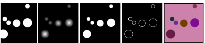
아래의 결과는 왼쪽순서대로 다음과 같다.
- src: 원본 사진
- dist:
cv2.distanceTransform()결과 - mask: dist의 결과를 선명하게 나타내기 위하여 특정 임계값 이상의 값을 255이상의 값을 갇도록 설정하였다.
- markers:
cv2.findContours(), cv2.drawContours()을 통하여 mask의 경계값을 찾아서 그리도록 하였다. 주요한 점은 i+1을 통해 각각의 경계값은 다른 값으로서 구분하였다. - dst:
cv2.watershed()와 markers의 각각 가중치를 주어 결과출력
참고사항
좀 더 정확한 동작원리와 예시에 대해서 궁금하면 아래 링크를 참조하자.
OpenCV 참조 설명
1
2
3
4
5
6
7
8
9
10
11
12
13
14
15
16
17
18
19
20
21
22
23
24
25
26
27
28
29
30
31
32
33
34
35
36
37
38
39
40
41
42
43
44
45
46
47
48
49
50
51
52
53
54
55
56
57
58
src = cv2.imread('./data/circle.jpg')
gray = cv2.cvtColor(src,cv2.COLOR_BGR2GRAY)
ret,bimage = cv2.threshold(gray,0,255,cv2.THRESH_BINARY_INV+cv2.THRESH_OTSU)
dist = cv2.distanceTransform(bimage,cv2.DIST_L1,3)
dist8 = cv2.normalize(dist,None,0,255,cv2.NORM_MINMAX,dtype=cv2.CV_8U)

minVal,maxVal,minLoc,maxLoc = cv2.minMaxLoc(dist)
print('dist:',minVal,maxVal,minLoc,maxLoc)
mask = (dist>maxVal*0.1).astype(np.uint8)*255

mode = cv2.RETR_EXTERNAL
method = cv2.CHAIN_APPROX_SIMPLE
contours,hierarchy = cv2.findContours(mask,mode,method)
print('len(contours)=',len(contours))

markers = np.zeros(shape=src.shape[:2],dtype=np.int32)

for i,cnt in enumerate(contours):
    cv2.drawContours(markers,[cnt],0,i+1,3)


dst = src.copy()
cv2.watershed(src,markers)

np.random.seed(0)

for i in range(len(contours)):
    r = np.random.randint(256)
    g = np.random.randint(256)
    b = np.random.randint(256)
    dst[markers==i+1] = [b,g,r]
dst = cv2.addWeighted(src,0.4,dst,0.6,0)

markers = np.zeros(shape=src.shape[:2],dtype=np.int32)
for i,cnt in enumerate(contours):
    cv2.drawContours(markers,[cnt],0,np.random.randint(150,256),3)


wImg_bimage = Image(layout = Layout(border="solid"), width="20%")
wImg_dist8 = Image(layout = Layout(border="solid"), width="20%")
wImg_mask = Image(layout = Layout(border="solid"), width="20%")
wImg_marker = Image(layout = Layout(border="solid"), width="20%")
wImg_dst = Image(layout = Layout(border="solid"), width="20%")

items = [wImg_bimage,wImg_dist8,wImg_mask,wImg_marker,wImg_dst]
box = Box(items)
display.display(box)

tmpStream = cv2.imencode(".jpeg", bimage)[1].tostring()
wImg_bimage.value = tmpStream
tmpStream = cv2.imencode(".jpeg", dist8)[1].tostring()
wImg_dist8.value = tmpStream
tmpStream = cv2.imencode(".jpeg", mask)[1].tostring()
wImg_mask.value = tmpStream
tmpStream = cv2.imencode(".jpeg", markers)[1].tostring()
wImg_marker.value = tmpStream
tmpStream = cv2.imencode(".jpeg", dst)[1].tostring()
wImg_dst.value = tmpStream
cv2.watershed() 영상 분할 결과
피라미드 기반 분할
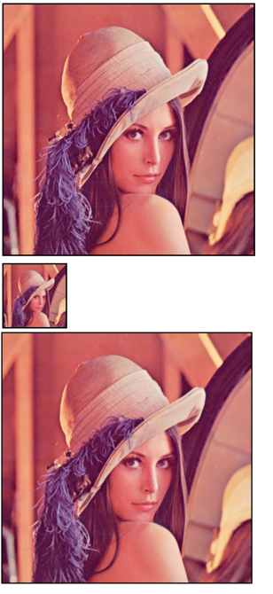
피라미드(Pyrimid)영상: 피라미드 영상이란 다양한 스케일에 걸쳐 영상을 나타내는 것 이다.

사진 출처:eehoeskrap
영상처리에 있어서 여러 스케일에 걸쳐 피라미드를 생성하여 처리를 하게 되면 물체를 비교하거나 매칭에 용이하게 쓸 수 있다. 예를들어 Object Detection에서 다른 스케일에서 동일한 객체인지 판단할 경우에 사용된다.
이러한 Image Pyramid는 (1)Gaussian Pyramids 와 (2) Laplacian Pyramids로 구분된다.
cv2.pyrDown(src[,dst[,dstsize[,borderType]]]): 가우시안 필터링 하고 dstsize에 주어진 크기로 축소한다.
parameter
- src: input
- dst: output
- dstsize: 축소할 크기
cv2.pyrUp(src[,dst[,dstsize[,borderType]]]): 가우시안 필터링 하고 dstsize에 주어진 크기로 확대한다.
parameter
- src: input
- dst: output
- dstsize: 확대할 크기
cv2.pyrDown(), cv2.pyrUp() (1) Gaussian Pyramid
1
2
3
4
5
6
7
8
9
10
11
12
13
14
15
16
17
18
19
20
21
22
23
24
src = cv2.imread('./data/lena.jpg')

down2 = cv2.pyrDown(src)
down4 = cv2.pyrDown(down2)
print('donw2.shape=',down2.shape)
print('down4.shape=',down4.shape)

up2 = cv2.pyrUp(src)
up4 = cv2.pyrUp(up2)
print('up2.shape=',up2.shape)
print('up4.shape=',up4.shape)

wImg_original = Image(layout = Layout(border="solid"))
wImg_down4 = Image(layout = Layout(border="solid"))
wImg_up4 = Image(layout = Layout(border="solid"))

display.display(wImg_original,wImg_down4,wImg_up4)

tmpStream = cv2.imencode(".jpeg", src)[1].tostring()
wImg_original.value = tmpStream
tmpStream = cv2.imencode(".jpeg", down4)[1].tostring()
wImg_down4.value = tmpStream
tmpStream = cv2.imencode(".jpeg", up4)[1].tostring()
wImg_up4.value = tmpStream
cv2.pyrDown(), cv2.pyrUp() (1) Gaussian Pyramid 결과
donw2.shape= (256, 256, 3)
down4.shape= (128, 128, 3)
up2.shape= (1024, 1024, 3)
up4.shape= (2048, 2048, 3)
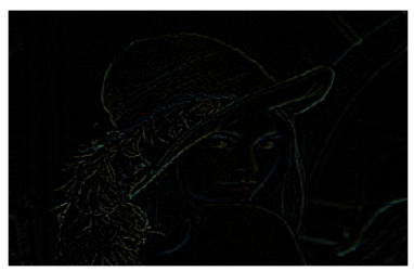
cv2.pyrDown(), cv2.pyrUp() (2) Laplacian Pyramid
Laplacian Pyramid는 Gaussian Pyramid에 의해서 생성된다.
cv2.pyrDown(), cv2.pyrUp()을 사용하여 축소, 확장을 하면 원본과 동일한 이미지를 얻을 수 없다.
만약 원본 이미지의 shape(255,400,3)을 cv2.pyrDown()을 적용하면 행과 열이 2배씩 줄게 되고 소수점은 반올림 되어 (113,200,3)이 된다.
이러한 결과를 다시 cv2.pyrUp()을 적용하면 (226,400,3)이된다.
이러한 차이는 1row차이를 발생하게 되어서 Edge를 검출할 수 있게된다.
1
2
3
4
5
6
7
8
9
10
11
12
13
14
15
16
17
18
19
20
img= cv2.imread('./data/lena.jpg')
print(img.shape)

img = cv2.resize(img,dsize=(400,255))
print(img.shape)

GAD = cv2.pyrDown(img)
print(GAD.shape)

GAU = cv2.pyrUp(GAD)
print(GAU.shape)

temp = cv2.resize(GAU,(400,255))
print(type(temp))
print(type(img))
print(temp.shape)
print(img.shape)
res = cv2.subtract(img,temp)
plt.axis('off')
plt.imshow(res)
cv2.pyrDown(), cv2.pyrUp() (2) Laplacian Pyramid 결과
(512, 512, 3)
(255, 400, 3)
(128, 200, 3)
(256, 400, 3)
<class ‘numpy.ndarray’>
<class ‘numpy.ndarray’>
(255, 400, 3)
(255, 400, 3)
cv2.pyrMeanShiftFiltering() 영역 검출
cv2.pyrMeanShiftFiltering(src, sp, sr[, dst[, maxLevel[, termcrit]]]): 영상에 피라미드 기반 평균이동(meanshifting)필터링을 수행한다.
parameter
- src: 3 channel의 input
- sp: 공간 윈도우의 크기
- sr: 컬러 윈도우의 크기
- maxLevel: 피라미드의 최고 Level
- termcrit: 피라미드 수행 종료 시기
- cv2.TERM_CRITERIA_MAX_ITER
- cv2.TERM_CRITERIA_MAX_COUNT
- cv2.TERM_CRITERIA_MAX_EPS
진행 과정
공간윈도우와 컬러 윈도우를 사용하여 반복적으로 meanshift를 수행한다.
1. 공간 위도우 내의 좌표 설정
$$X-sp \leq x \leq X+sp$$
$$Y-sp \leq y \leq Y+sp$$
2. 컬러 윈도우 내의 값 설정
$$|(R,G,B) - (r,g,b)| \leq sr$$
3. 결과값 저장
$$dst(X,Y) = (R^{*},G^{*},B^{*})$$
아래 Code는 flower.jpg에 대한 RGB, HSV의 meanshifting Filtering의 결과이다.
floodFillPostProcess(): 원본 이미지에 대하여 비슷한 주변 pixel끼리의 segmentation구행하는 Method
sp, sr, maxLevel을 바꿔가면서 결과를 바로바로 확인할 수 있도록 ipywidget으로 구성하였다.
1
2
3
4
5
6
7
8
9
10
11
12
13
14
15
16
17
18
19
20
21
22
23
24
25
26
27
28
29
30
31
32
33
34
35
36
37
38
39
40
41
42
43
44
45
46
47
48
49
50
51
52
53
54
55
56
57
58
59
60
61
62
63
64
65
66
67
68
69
70
71
72
73
74
75
76
77
78
79
80
81
82
83
84
85
86
87
88
89
90
91
92
93
94
95
96
97
98
99
100
101
102
103
104
105
106
107
108
109
110
111
112
113
114
115
116
117
118
119
120
121
122
123
124
125
126
127
128
129
130
131
132
133
134
135
136
137
138
139
140
141
142
143
144
145
146
147
148
149
150
151
152
153
154
155
156
157
158
159
160
161
162
163
164
165
166
167
168
169
170
171
172
173
174
175
176
177
178
179
180
181
182
183
184
185
186
187
188
189
190
191
192
193
194
195
196
197
198
199
200
201
202
203
204
205
206
207
208
209
210
211
212
213
214
215
216
217
218
219
220
221
222
223
224
def floodFillPostProcess(src,diff=(2,2,2)):
    img = src.copy()
    rows,cols = img.shape[:2]
    mask = np.zeros(shape=(rows+2,cols+2),dtype=np.uint8)
    for y in range(rows):
        for x in range(cols):
            if mask[y+1,x+1] == 0:
                r = np.random.randint(256)
                g = np.random.randint(256)
                b = np.random.randint(256)
                cv2.floodFill(img,mask,(x,y),(b,g,r),diff,diff)
    return img

src = cv2.imread('./data/flower.jpg')
hsv = cv2.cvtColor(src,cv2.COLOR_BGR2HSV)
dst = floodFillPostProcess(src)
dst2 = floodFillPostProcess(hsv)

#Component 선언
IntSlider_sp1 = IntSlider(
    value=0,
    min=0,
    max=30,
    step=1,
    description='sp: ',
    disabled=False,
    continuous_update=False,
    orientation='horizontal',
    readout=True,
    readout_format='d'
)

IntSlider_sr1 = IntSlider(
    value=0,
    min=0,
    max=30,
    step=1,
    description='sr: ',
    disabled=False,
    continuous_update=False,
    orientation='horizontal',
    readout=True,
    readout_format='d'
)

IntSlider_maxLevel1 = IntSlider(
    value=0,
    min=0,
    max=20,
    step=1,
    description='maxLevel: ',
    disabled=False,
    continuous_update=False,
    orientation='horizontal',
    readout=True,
    readout_format='d'
)

IntSlider_sp2 = IntSlider(
    value=0,
    min=0,
    max=30,
    step=1,
    description='sp: ',
    disabled=False,
    continuous_update=False,
    orientation='horizontal',
    readout=True,
    readout_format='d'
)

IntSlider_sr2 = IntSlider(
    value=0,
    min=0,
    max=30,
    step=1,
    description='sr: ',
    disabled=False,
    continuous_update=False,
    orientation='horizontal',
    readout=True,
    readout_format='d'
)

IntSlider_maxLevel2 = IntSlider(
    value=0,
    min=0,
    max=5,
    step=1,
    description='maxLevel: ',
    disabled=False,
    continuous_update=False,
    orientation='horizontal',
    readout=True,
    readout_format='d'
)

def layout(header, left, right):
    layout = AppLayout(header=header,
          left_sidebar=left,
          center=None,
          right_sidebar=right)
    return layout

wImg_original = Image(layout = Layout(border="solid"), width="50%")
wImg_hsv = Image(layout = Layout(border="solid"), width="50%")
wImg_original_floodFill = Image(layout = Layout(border="solid"), width="50%")
wImg_hsv_floodFill = Image(layout = Layout(border="solid"), width="50%")

wImg_res1 = Image(layout = Layout(border="solid"), width="50%")
wImg_dst1 = Image(layout = Layout(border="solid"), width="50%")

wImg_res2 = Image(layout = Layout(border="solid"), width="50%")
wImg_dst2 = Image(layout = Layout(border="solid"), width="50%")

items = [wImg_original,wImg_original_floodFill]
items2 = [wImg_hsv,wImg_hsv_floodFill]
floodFill1 = Box(items)
floodFill2 = Box(items2)
box1 = layout(None,floodFill1,floodFill2)

items = [IntSlider_sp1,IntSlider_sr1,IntSlider_maxLevel1]
trick_bar = Box(items)
box2 = layout(trick_bar,wImg_res1,wImg_dst1)

items = [IntSlider_sp2,IntSlider_sr2,IntSlider_maxLevel2]
trick_bar = Box(items)
box3 = layout(trick_bar,wImg_res2,wImg_dst2)

tab_nest = widgets.Tab()
tab_nest.children = [box1, box2, box3]
tab_nest.set_title(0, 'floodFill')
tab_nest.set_title(1, 'src 영역 검출')
tab_nest.set_title(2, 'hsv 영역 검출')
tab_nest

display.display(tab_nest)

#box1 값 대입
tmpStream = cv2.imencode(".jpeg", src)[1].tostring()
wImg_original.value = tmpStream
tmpStream = cv2.imencode(".jpeg", hsv)[1].tostring()
wImg_hsv.value = tmpStream
tmpStream = cv2.imencode(".jpeg", dst)[1].tostring()
wImg_original_floodFill.value = tmpStream
tmpStream = cv2.imencode(".jpeg", dst2)[1].tostring()
wImg_hsv_floodFill.value = tmpStream

sp1,sr1,maxLevel1 = 0,0,0
sp2,sr2,maxLevel2 = 0,0,0

#box2,3값 대입
def input_box_value(option=1):
    global sp1,sr1,maxLevel1,sp2,sr2,maxLevel2
    input_sp,input_sr,input_maxLevel,res = 0,0,0,0

    if option == 1:
        input_sp = sp1
        input_sr = sr1
        input_maxLevel = maxLevel1
        res = cv2.pyrMeanShiftFiltering(src,sp=input_sp,sr=input_sr,maxLevel=input_maxLevel)
    else:
        input_sp = sp2
        input_sr = sr2
        input_maxLevel = maxLevel2
        term_crit = (cv2.TERM_CRITERIA_MAX_ITER,10,2)
        res = cv2.pyrMeanShiftFiltering(hsv,sp=input_sp,sr=input_sr,maxLevel=input_maxLevel,termcrit=term_crit)
    dst = floodFillPostProcess(res)
    tmpStream = cv2.imencode(".jpeg", res)[1].tostring()
    tmpStream2 = cv2.imencode(".jpeg", dst)[1].tostring()

    if option == 1:
        wImg_res1.value = tmpStream
        wImg_dst1.value = tmpStream2
    else:
        wImg_res2.value = tmpStream
        wImg_dst2.value = tmpStream2

#Event 선언
def on_value_change_sp1(change):
    global sp1,sr1,maxLevel1
    sp1 = change['new']
    input_box_value()


def on_value_change_sr1(change):
    global sp1,sr1,maxLevel1
    sr1 = change['new']
    input_box_value()

def on_value_change_maxLevel1(change):
    global sp1,sr1,maxLevel1
    maxLevel1 = change['new']
    input_box_value()

def on_value_change_sp2(change):
    global sp2,sr2,maxLevel2
    sp2 = change['new']
    input_box_value(0)


def on_value_change_sr2(change):
    global sp2,sr2,maxLevel2
    sr2 = change['new']
    input_box_value(0)

def on_value_change_maxLevel2(change):
    global sp2,sr2,maxLevel2
    maxLevel2 = change['new']
    input_box_value(0)

#초기화 작업
input_box_value()
input_box_value(0)


#Component에 Event 장착
IntSlider_sp1.observe(on_value_change_sp1, names='value')
IntSlider_sr1.observe(on_value_change_sr1, names='value')
IntSlider_maxLevel1.observe(on_value_change_maxLevel1, names='value')

IntSlider_sp2.observe(on_value_change_sp2, names='value')
IntSlider_sr2.observe(on_value_change_sr2, names='value')
IntSlider_maxLevel2.observe(on_value_change_maxLevel2, names='value')
cv2.pyrMeanShiftFiltering() 영역 검출 결과
기본 결과(sp=0, sr=0, maxLevel=0)
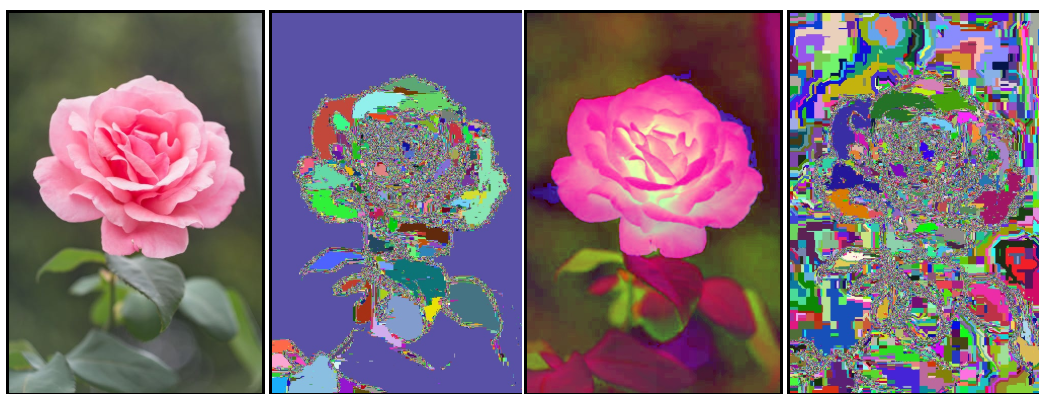
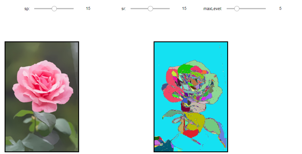
src 영역 검출(sp=15, sr=15, maxLevel=5)
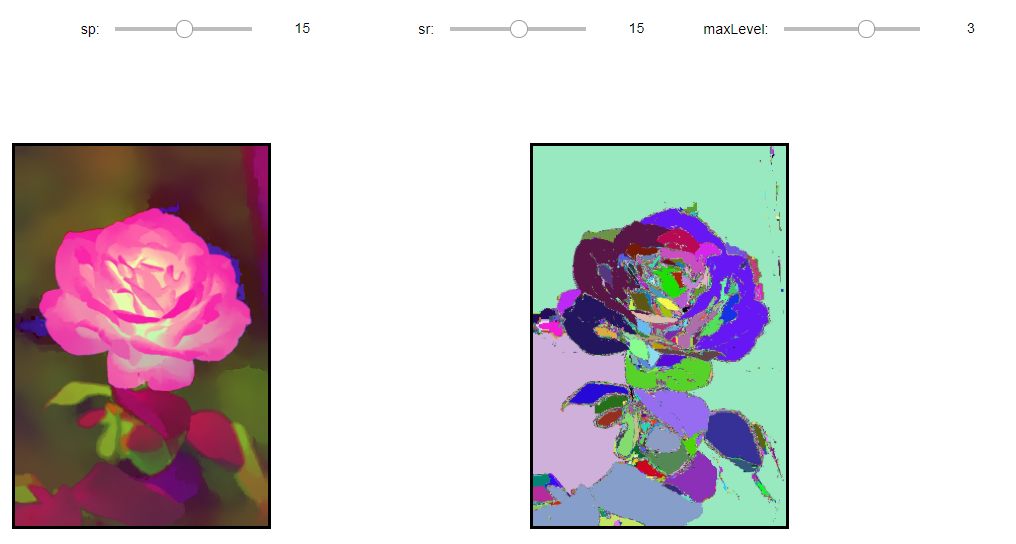
hsv 영역 검출(sp=15, sr=15, maxLevel=3)
K-Means 클러스터링 분할
K-Means Clusturing은 분리형 군집화 알고리즘중 하나로서, 각 군집은 하나의 중심을 가지고 각 개체는 가장 가까운 중심에 할당되며, 같은 중심에 개체들이 모여 하나의 군집을 형성하는 방법이다.
이러한 방식은 사전에 군집 수(k)를 사용자가 지정해야하는 hyperparameter이다.
학습 과정
1. 클러스터 개수 K를 고정하고, t=0으로 초기화 한다. K 개의 클러스터( \(C^{0}_{i}, i=1, ..., K\))의 평균(\(m^{0}_{i}, i=1, ..., K\))을 임의로 선택한다.

2. 클러스터링하려는 데이터(\(x_{j}, j=1, ..., M\))각각의 K개의 클러스터 평균과의 최소거리가 되는 클러스터(\(C^{t}_{p}\))로 \(x_{j}\)를 분류

3. 각 클러스터(\(C^{t}_{i}, i=1, ..., K\))에 속한 데이터를 이용하여 새로운 클러스터 평균 \(m^{t+1}_{i}, i=1, ..., K\) 을 계산한다.
$$m^{t+1}_{i} = \frac{1}{C^{t}_{i}} \sum_{x \in C^{t}_{i}}x_{j}, i=1, ..., K$$

4. t = t+1로 증가시키고 최대 반복회수까지 2~3단계를 계속하여 반복한다.
2단계 반복

3단계 반복

장점 및 단점
장점: 계산 복잡성이 O(n)이여서 가벼운 편이다.
단점:
- 군집의 크기가 다를 경우 제대로 작동하지 않을 수 있다.

- 군집의 밀도가 다를 경우 제대로 작동하지 않을 수 있다.

- 데이터 분포가 특이한 케이스인 경우 제대로 작동하지 않을 수 있다.

그림 출처: ratsgo 블로그
cv2.kmeans(data,K,bestLabels,criteria,attemps,flags[,centers]): K-means클러스터링 수행
parameter
- src: input
- K: 클러스터 개수
- criteria: 반복 회수 종료 시점 정의
- ateempts: 알고리즘 시도하는 회수, 서로다른 시도 횟수 중 최적을 레이블링 경과를 bestLabels에 저장하여 반환
- flags: K개의 클러스터 중심을 초기화하는 방법을 명시한다.
- cv2.KMEANS_RANDOM_CENTERS: 난수를 사용하여 설정
- cv2.KMEANS_PP_CENTERS: Arthur and Vassivitskii에 의해 제안 방법
- cv2.KMEANS_USE_INITIAL_LABELS: 처음 시도에는 사용자가 제공한 레이블을 사용하고, 다음 시도부터는 난수를 이용하여 임의로 설정
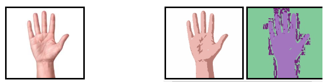
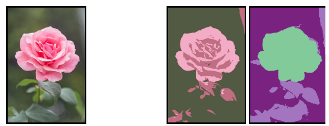
컬러 클러스터링 영역 검출
각각의 hand.jpg와 flower.jpg에 대하여 bgr, hsv에 대해 각각 3개의 군집으로 K-means Clustering한 결과 이다.
1
2
3
4
5
6
7
8
9
10
11
12
13
14
15
16
17
18
19
20
21
22
23
24
25
26
27
28
29
30
31
32
33
34
35
36
37
38
39
40
41
42
43
44
45
46
47
48
49
50
51
52
53
54
55
56
57
58
59
60
61
62
63
64
65
66
67
68
69
70
71
72
73
74
75
76
77
78
79
80
81
82
83
84
85
86
87
88
89
90
91
92
93
94
95
96
97
98
99
100
101
102
103
104
105
106
107
108
109
110
111
112
113
114
115
116
117
118
src1 = cv2.imread('./data/hand.jpg')
src2 = cv2.imread('./data/flower.jpg')

hsv1 = cv2.cvtColor(src1,cv2.COLOR_BGR2HSV)
hsv2 = cv2.cvtColor(src2,cv2.COLOR_BGR2HSV)

data1 = src1.reshape((-1,3)).astype(np.float32)
data2 = src2.reshape((-1,3)).astype(np.float32)

data3 = hsv1.reshape((-1,3)).astype(np.float32)
data4 = hsv2.reshape((-1,3)).astype(np.float32)

K = 3
term_crit = (cv2.TERM_CRITERIA_EPS+cv2.TERM_CRITERIA_MAX_ITER,10,1.0)

ret1,labels1,centers1 = cv2.kmeans(data1,K,None,term_crit,5,cv2.KMEANS_RANDOM_CENTERS)
print('bgr')
print('hand.jpg')
print('centers.shape=',centers1.shape)
print('labels.shape=',labels1.shape)
print('ret=',ret1)
print('-'*20)

ret2,labels2,centers2 = cv2.kmeans(data2,K,None,term_crit,5,cv2.KMEANS_RANDOM_CENTERS)
print('flower.jpg')
print('centers.shape=',centers2.shape)
print('labels.shape=',labels2.shape)
print('ret=',ret)

print('*'*20)
ret3,labels3,centers3 = cv2.kmeans(data3,K,None,term_crit,5,cv2.KMEANS_RANDOM_CENTERS)
print('hsv')
print('hand.jpg')
print('centers.shape=',centers3.shape)
print('labels.shape=',labels3.shape)
print('ret=',ret3)
print('-'*20)

ret4,labels4,centers4 = cv2.kmeans(data4,K,None,term_crit,5,cv2.KMEANS_RANDOM_CENTERS)
print('flower.jpg')
print('centers.shape=',centers4.shape)
print('labels.shape=',labels4.shape)
print('ret=',ret4)


centers1 = np.uint8(centers1)
res1 = centers1[labels1.flatten()]
bgr1 = res1.reshape(src1.shape)

centers2 = np.uint8(centers2)
res2 = centers2[labels2.flatten()]
bgr2 = res2.reshape(src2.shape)


labels3 = np.uint8(labels3.reshape(src1.shape[:2]))
labels4 = np.uint8(labels4.reshape(src2.shape[:2]))

dst3 = np.zeros(src1.shape,dtype=src1.dtype)
dst4 = np.zeros(src2.shape,dtype=src2.dtype)

for i in range(K):
    r = np.random.randint(256)
    g = np.random.randint(256)
    b = np.random.randint(256)
    dst3[labels3 ==i] = [b,g,r]
    dst4[labels4 ==i] = [b,g,r]

hsv1 = dst3
hsv2 = dst4


def layout(header, left, right):
    layout = AppLayout(header=header,
          left_sidebar=left,
          center=None,
          right_sidebar=right)
    return layout

wImg_original1 = Image(layout = Layout(border="solid"), width="50%")
wImg_bgr1 = Image(layout = Layout(border="solid"), width="50%")
wImg_hsv1 = Image(layout = Layout(border="solid"), width="50%")

wImg_original2 = Image(layout = Layout(border="solid"), width="50%")
wImg_bgr2 = Image(layout = Layout(border="solid"), width="50%")
wImg_hsv2 = Image(layout = Layout(border="solid"), width="50%")

items = [wImg_bgr1,wImg_hsv1]
Clustering = Box(items)
box1 = layout(None,wImg_original1,Clustering)

items = [wImg_bgr2,wImg_hsv2]
Clustering = Box(items)
box2 = layout(None,wImg_original2,Clustering)

tab_nest = widgets.Tab()
tab_nest.children = [box1, box2]
tab_nest.set_title(0, 'Clustering1(BGR, HSV)')
tab_nest.set_title(1, 'Clustering2(BGR, HSV)')
tab_nest

display.display(tab_nest)

#box1 값 대입
tmpStream = cv2.imencode(".jpeg", src1)[1].tostring()
wImg_original1.value = tmpStream
tmpStream = cv2.imencode(".jpeg", bgr1)[1].tostring()
wImg_bgr1.value = tmpStream
tmpStream = cv2.imencode(".jpeg", hsv1)[1].tostring()
wImg_hsv1.value = tmpStream

#box2 값 대입
tmpStream = cv2.imencode(".jpeg", src2)[1].tostring()
wImg_original2.value = tmpStream
tmpStream = cv2.imencode(".jpeg", bgr2)[1].tostring()
wImg_bgr2.value = tmpStream
tmpStream = cv2.imencode(".jpeg", hsv2)[1].tostring()
wImg_hsv2.value = tmpStream
컬러 클러스터링 영역 검출 결과
hand.jpg
flower.jpg
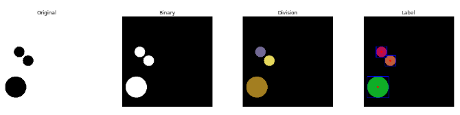
연결요소 검출
cv2.threshold(), cv2.inRange()등으로 생성한 이진 영상에서 4-이웃 또는 8-이웃 연결성을 고려하여 연결요소를 라벨링하여 BLOB(binary Large Object)영역을 검출한다.
cv2.connectedComponents(image[,labels[,connectivity[,itype]]]): 연결된 components의 개수를 반환하고 Labeling을 해준다.
parameter
- image: input
- labels: output
- connectivity: 4 or 8이웃 연결성
- itype: output image label type
cv2.connectedComponentsWithStats(image[,labels[,stats[,centroids[,connectivity[,itype]]]]]): 위의 기능 및 중심 좌표 및 범위를 알려주기 때문에 Component를 특정화 시킬 수 있다.
return
- stats: x,y,width,height,area
- centroids: 중심 좌표
주의사항
OpenCV에서 제공하는 cv.connectedComponents(), cv2.connectedComponentsWithStats는 이진 영상에서 검은색을 Background, 흰색을 연결대상으로 Mapping한다.
1
2
3
4
5
6
7
8
9
10
11
12
13
14
15
16
17
18
19
20
21
22
23
24
25
26
27
28
29
30
31
32
33
34
35
36
37
38
39
40
41
42
43
44
45
46
47
48
49
50
51
52
53
54
55
src = cv2.imread('./data/circle2.jpg')
gray = cv2.cvtColor(src,cv2.COLOR_BGR2GRAY)
ret,res = cv2.threshold(gray,128,255,cv2.THRESH_BINARY_INV)

ret,labels = cv2.connectedComponents(res)
print('ret=',ret)

dst = np.zeros(src.shape,dtype=src.dtype)

for i in range(1,ret):
    r = np.random.randint(256)
    g = np.random.randint(256)
    b = np.random.randint(256)
    dst[labels == i] = [b,g,r]

ret2,labels2,stats,centroids = cv2.connectedComponentsWithStats(res)
print('ret2=',ret2)
print('stats=',stats)
print('centroids',centroids)

dst2 = np.zeros(src.shape,dtype=src.dtype)

for i in range(1,int(ret2)):
    r = np.random.randint(256)
    g = np.random.randint(256)
    b = np.random.randint(256)
    dst2[labels2 == i] = [b,g,r]

for i in range(1,int(ret2)):
    x,y,width,height,area = stats[i]
    cv2.rectangle(dst2,(x,y),(x+width,y+height),(0,0,255),2)
    cx,cy = centroids[i]
    cv2.circle(dst2,(int(cx),int(cy)),5,(255,0,0),-1)


plt.figure(figsize=(20,4))
imgae1=plt.subplot(1,4,1)
imgae1.set_title('Original')
plt.axis('off')
plt.imshow(src)

imgae2=plt.subplot(1,4,2)
imgae2.set_title('Binary')
plt.axis('off')
plt.imshow(res, cmap="gray")

imgae3=plt.subplot(1,4,3)
imgae3.set_title('Division')
plt.axis('off')
plt.imshow(dst)

imgae3=plt.subplot(1,4,4)
imgae3.set_title('Label')
plt.axis('off')
plt.imshow(dst2)
연결요소 검출 결과
ret= 4
ret2= 4
stats= [[     0      0    512    512 245213]
 [    70    170     61     61   2821]
 [   120    220     61     61   2821]
 [    20    340    121    121  11289]]
centroids [[266.58220404 249.54933874]
 [100.         200.        ]
 [150.         250.        ]
 [ 80.         400.        ]]
참조:원본코드
참조:Python으로 배우는 OpenCV 프로그래밍
문제가 있거나 궁금한 점이 있으면 wjddyd66@naver.com으로 Mail을 남겨주세요.
Leave a comment