Paper32. MLDRL: Multi-loss disentangled representation learning for predicting esophageal cancer response to neoadjuvant chemoradiotherapy using longitudinal CT images

MLDRL: Multi-loss disentangled representation learning for predicting esophageal cancer response to neoadjuvant chemoradiotherapy using longitudinal CT images

• Paper: MLDRL: Multi-loss disentangled representation learning for predicting esophageal cancer response to neoadjuvant chemoradiotherapy using longitudinal CT images
• Code: yuehailin GitHub

Abbreviation

• pCR (prediction of pathological complete response): 화학방사선요법 완료 후 암이 사라지는 것 (e.g. Pegah et al.: Pathological complete response (pCR) is defined as disappearance of all invasive cancer in the breast after completion of neoadjuvant chemotherapy.)
• nCRT (neoadjuvant chemoradiothera): 화학방사선요법

Abstract

Accurate prediction of pathological complete response (pCR) after neoadjuvant chemoradiotherapy (nCRT) is essential for clinical precision treatment. However, the existing methods of predicting pCR in esophageal cancer are based on the single stage data, which limits the performance of these methods. Effective fusion of the longitudinal data has the potential to improve the performance of pCR prediction, thanks to the combination of complementary information. In this study, we propose a new multi-loss disentangled representation learning (MLDRL) to realize the effective fusion of complementary information in the longitudinal data. Specifically, we first disentangle the latent variables of features in each stage into inherent and variational components. Then, we define a multi-loss function to ensure the effectiveness and structure of disentanglement, which consists of a cross-cycle reconstruction loss, an inherent-variational loss and a supervised classification loss. Finally, an adaptive gradient normalization algorithm is applied to balance the training of multiple loss terms by dynamically tuning the gradient magnitudes. Due to the cooperation of the multi-loss function and the adaptive gradient normalization algorithm, MLDRL effectively restrains the potential interference and achieves effective information fusion. The proposed method is evaluated on multi-center datasets, and the experimental results show that our method not only outperforms several state-of-art methods in pCR prediction, but also achieves better performance in the prognostic analysis of multi-center unlabeled datasets.

해당 논문에서는 esophageal cancer의 정확한 예측을 하기 위하여 single modality가 아닌 multi-modality(CT images before nCRT + CT images after nCRT)로서 예측할 수 있는 모델을 제안한다. 제안하는 모델 MLDRL은 각각의 modality에서 공통적인 요소인 inherent과 개별적인 요소인 variational component로서 disentangle한다. 그뒤, 여러 Loss와 adaptive gradient normalization algorithm을 활용하여 제안하는 model을 학습하고 성능을 보여준다.

Dataset

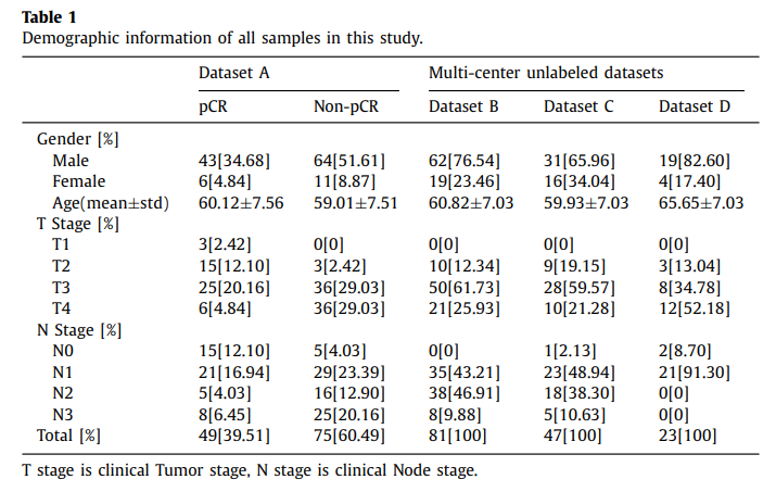
• Dataset A: (1) 모든 환자는 식도암. (2) 모든 환자는 nCRT 치료 받음. (3) 모든 환자는 식도절제술 받음. (4) 수술후 절제된 표본에서 histopathological examination수행
• Dataset B, C, D: (1) 모든 환자는 식도암. (2) 모든 환자는 nCRT 치료 받음. (3) 모든 환자는 실도절제술 받음. (4) 모든 환자의 prognostic information (survival time and survival statue)은 사용 가능. (하지만, pCR의 정보는 몇몇 환자가 없어, unlabeled dataset으로 분류됨.)

Dataset Preprocessing의 경우 MIACSU로서 자신들이 개발한 Tool로서 진행하였고, Preprocessing 후 2153개의 Feature중에서 81개의 Feature를 Random Forest로서 선택하였다.

Methods

Structure & Experiment Setting

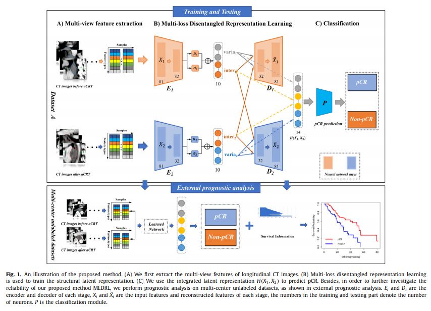
해당 논문에서는 크게 2가지 Stage로서 실험을 구성하였다. 처음은, 모든 Label 정보 (pCR or Non-pCR)가 있는 Dataset A로서 Model을 학습하고 Classification Performance를 비교하였다.
그 다음, 학습된 model을 가지고 unlabel을 포함한 Dataset B, C, D로서 external prognostic analysis을 수행하였다.

Structure for latent representation

아래에서 사용한 Loss는 대부분 선행연구인 DME-AEE와 비슷하므로 간략히 설명하고 넘어간다.

Notation

• \(N\): Number of samples
• \(M\): Number of modality
• \(X_i\): i-th modality
• \(E_i\): i-th encoder
• \(D_i\): i-th decoder
• \(Y_n^{(m)}\): n-th sample for class m

Cross-cycle reconstruction loss.
GAN의 수식은 간략히 표현하면 아래와 같다.

$$\text{Loss}_{\text{vae}}(\phi, \theta) = -\mathbb{E}_{Z \sim q_{\phi}(Z|X)}[\log p_{\theta}(X|Z)] + KL(q_{\phi}(Z|X) || p_{\theta}(Z))$$

해당 저자들은 위의 수식을 활용하여, DME-AEE와 마찬가지로 공통적인 (inher)요소를 강조하여 학습하는 것을 목표로한다. 따라서 아래와 같이 i-th modality를 reconstruction하는데 i-th specific + j-th common으로서 reconstruction되는 cross-cycle reconstruction loss를 사용한다.

$$\text{Loss}_{\text{recon}} = \sum_{i=1}^{2} \sum_{j=1}^{2} \| X_i - D_i(\text{Inher}(E_j (X_j)), \text{Varia}(E_i (X_i)))\|^2 + KL(q_{\phi}(Z_i|X_i) || p_{\theta}(Z_i))$$

Inherent-variational loss
DME-AEE와 동일하게 공통적인 부분은 같을수록, 다른 부분은 다를 수록 Loss가 작아지게 구성한다.

$$\text{Loss}_{\text{inher-varia}} = \frac{\text{Loss}_{\text{inher}}}{\text{Loss}_{\text{varia}}}$$

$$\text{Loss}_{\text{inher}} = \| \text{Inher}(E_1(X_1)), \text{Inher}(E_2(X_2)) \|_2$$

$$\text{Loss}_{\text{varia}} = \| \text{Varia}(E_1(X_1)), \text{Varia}(E_2(X_2)) \|_2$$

Supervised classification loss.
Classfication에서 많이 사용하는 Cross Entropy Loss를 사용하였다.

$$\text{Loss}_{\text{class}} = -\frac{1}{N} =\sum_{n=1}^{N} \sum_{m=1}^{M} Y_n^{(m)} \log \hat{Y}_n^{(m)}$$

Classification에 들어가는 Input은 아래와 같이 구성된다.

$$H(X_1, X_2) = [\text{inherent}_{1,2}, \text{variational}_1, \text{variational}_2]$$

$$\text{inherent}_{1,2} = \frac{1}{2}(\text{inherent}_{1} + \text{inherent}_2)$$

Joint loss
위의 모든 Loss를 weights를 주어 학습한다.

$$\text{Loss}_{\text{joint}} = \lambda \text{Loss}_{\text{recon}}+ \beta \text{Loss}_{\text{inher-varia}}+ \gamma \text{Loss}_{\text{class}}$$

Adaptive gradient normalization algorithm for optimization

기존의 DME-AEE와 다른 점 이다.
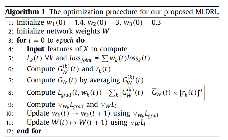
해당 논문에서 문제점으로 삼은 것은 최종적인 Loss Function의 \(\text{Loss}_{\text{joint}}\)가 3개의 multi-loss를 사용하므로 optimization을 하기 힘들 뿐만 아니라, magnitude도 모두 다르다는 것을 알 수 있다. 이러한 문제점을 해결하기 위하여 adaptive gradient normalization을 사용하여 parameter인 \(\lambda, \beta, \gamma\)의 값을 조절하는 방법을 사용하였다.

먼저, 최종적인 Loss (\(\text{Loss}_{\text{joint}}\))를 간략히 표현하면 아래와 같다.

$$\text{Loss}_{\text{joint}} = \sum w_k(t) \text{Loss}_{k}(t)$$

$$w_k(t): \text{Adaptive weight}, t: \text{epoch(=step)}$$

위의 Loss에서 Adaptive weights인 \(w_k(t)\)를 조절하여, balance되고 converge되게 학습하는 방법을 소개하기 위하여 아래와 같이 variable을 먼저 정의한다.

• \(G_w^{(k)} = \| \nabla w_k(t)L_k(t) \|_2\): \(L_2\) norm of the gradient of the wieghted k-th loss(\(w_k(t)L_k(t)\))
• \(\bar{G}_w(t) = E_{task} [G_w^{(k)}(t)]\): Average gradient norm in all losses at step t
• \(L_k (0)\): k-th loss value at step 0
• \(L_k (t)\): k-th loss value at step t
• \(\tilde{L}_k = L_k (t) / L_k (0)\): the inverse training rate of the k-th loss at step t
• \(r_k(t) = \tilde{L}_k(t) / E_{task}[\tilde{L}_k]\): relative inverse training rate for k-th loss at step t

위와같이 정의하였을 때, desired gradient norm은 아래와 같이 정의할 수 있다.

$$G_w^{(k)}(t) \mapsto \bar{G}_w(t) x [r_k(t)]^{\alpha}$$

$$\alpha: \text{Extra Hyperparameter (0.16 in paper)}, \mapsto: \text{actual function mapping.}$$

위의 정의한 notation을 활용하여 최종적인 adaptive gradient normalization의 식은 아래와 같고, Algirhm 1에 자세히 설명되어있다.

$$L_{grad}(t;w_k(t)) = \sum_{k} | G_w^{(k)}(t) - \bar{G}_w(t) x [r_k(t)]^{\alpha}|$$

Appendix. Adaptive gradient normalization
Adaptive gradient normalization에 대한 개인적인 생각입니다. 위의 Loss를 보고 개인적으로는 Adagrad와 매우 비슷한 formulation을 가지는 수식이라고 생각하였습니다.
먼저, Adagrad의 식을 살펴보면 아래와 같이 적을 수 있습니다.

$$\theta_{t} = \theta_{t-1} -\alpha \frac{g_t}{\sqrt{\sum_{i=1}^t g_i^2}}$$

위의 수식을 살펴보게 되면, update가 많이 된 parameter들은 optimum에 거의 도달했다고 생각하여 stepsize를 줄여서 update를 진행하고, update가 적게 된 parameter들은 optimum까지의 가야할 길이 멀다고 생각하여 stepsize를 크게 주는 optimization방법이라고 생각하면 된다.

해당 논문에서 Adaptive gradient normalization를 사용한 이유는 각각의 Loss가 비슷하게 수렴하게 하기 위해서 이다. 여기서 개인적으로 고려해야 할 사항은 개개의 Loss관점에서 update되는 비율을 맞춰야 된다.

위의 사실을 기억하고 다시 최종적인 Loss를 살펴보면 아래와 같다.

$$L_{grad}(t;w_k(t)) = \sum_{k} | G_w^{(k)}(t) - \bar{G}_w(t) x [r_k(t)]^{\alpha}|$$

위의 수식을 각각의 Term으로서 살펴보면 아래와 같은 의미를 가지는 것을 알 수 있다.

• \(G_w^{(k)}(t)\): 기본적으로 Update되는 Loss
• \([r_k(t)]^{\alpha}\): 개개의 Loss관점에서도 update되는 비율을 맞춤, 각각의 Loss관점에서 처음에 비하여 Update가 얼만큼 되는지 파악하여 속도를 맞추게 된다. 처음에 비하여 비율로 보는 이유는 각각의 Loss별로 종류도 다르고 값의 차이가 있을 거기 때문에 절대적인 값으로서는 비교가 불가능 하기 때문이다.
• \(\bar{G}_w(t)\): Loss의 평균으로서 training초기에는 작은값이고, training이 진행할 수록 점차 큰 값을 가지게 된다. \([r_k(t)]^{\alpha}\) term은 비율을 의미하므로, 왜 사용하는지는 모르겠습니다. (\(G_w^{(k)}(t)\)여도 상관없다고 생각합니다. Supplementary에도 적혀있지 않았고, Converge하기 위해서 사용한지도 잘 모르겠습니다.)

Experiments and results

Classification

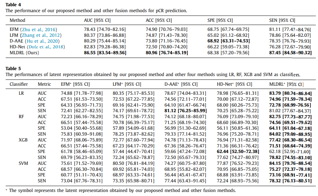
해당 논문에서는 Classification의 성능을 크게 2가지로 보여주었다. 첫번째로는 State-of-art model들과의 performance를 비교한 것 이였고, 두번째로는 Embedding에 machine learning classifier로서 성능을 비교한 것 이다. 위의 두가지 결과 모두 성능이 좋았고, 이는 model의 classification의 성능이 좋을 뿐만 아니라, classifier만으로 성능이 좋아진 것이 아니라 multi-modal에서 classification의 성능을 반영하여 embedding하는 것을 알 수 있다.

Ablation study

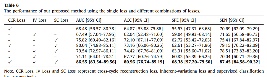
또한, Ablation study결과 사용한 3가지의 Loss 모두 Classification에 성능 향상에 도움이 되는 것을 알 수 있다.

Effect of multi-modal

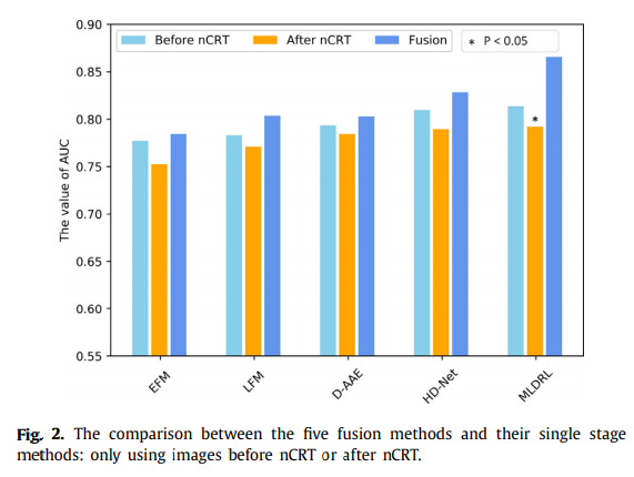
또한, 논문에서 제시하는 model은 multi-modal로서 performance를 높일 수 있는 것을 알 수 있다.

Pytorch Code

Model

• Normal: \(p_{\theta}(Z)\)
• Encoder1: \(E_1\)
• Decoder1: \(D_1\)
• Encoder2: \(E_2\)
• Decoder2: \(D_2\)

class Normal(object):
    def __init__(self, mu, sigma, log_sigma, v=None, r=None):
        self.mu = mu
        self.sigma = sigma  # either stdev diagonal itself, or stdev diagonal from decomposition
        self.logsigma = log_sigma
        dim = mu.get_shape()
        if v is None:
            v = torch.FloatTensor(*dim)
        if r is None:
            r = torch.FloatTensor(*dim)
        self.v = v
        self.r = r


class Encoder1(torch.nn.Module):
    def __init__(self, D_in, H):
        super(Encoder1, self).__init__()
        self.linear1 = torch.nn.Linear(D_in, H)

    def forward(self, x):

        return F.relu(self.linear1(x))


class Decoder1(torch.nn.Module):
    def __init__(self, latent, H, D_out):
        super(Decoder1, self).__init__()
        self.linear1 = torch.nn.Linear(latent, H)
        self.linear2 = torch.nn.Linear(H, D_out)
    def forward(self, x):
        x = F.relu(self.linear1(x))
        return F.relu(self.linear2(x))


class Encoder2(torch.nn.Module):
    def __init__(self, D_in, H):
        super(Encoder2, self).__init__()
        self.linear1 = torch.nn.Linear(D_in, H)

    def forward(self, x):

        return F.relu(self.linear1(x))


class Decoder2(torch.nn.Module):
    def __init__(self, latent, H, D_out):
        super(Decoder2, self).__init__()
        self.linear1 = torch.nn.Linear(latent, H)
        self.linear2 = torch.nn.Linear(H, D_out)

    def forward(self, x):
        x = F.relu(self.linear1(x))
        return F.relu(self.linear2(x))

Model

• h_enc1 = self.encoder1(x1): \(E_1(X_1)\)
• z1, mu1, sigma1 = self._sample_latent(h_enc1): reparameterize
• comm1, spe1 = z1.split([6,4], dim=1): \(\text{comm1}=(\text{Inher}(E_1 (X_1)), \text{spe1}=(\text{Varia}(E_1 (X_1))\)
• h_enc2 = self.encoder2(x2): \(E_2(X_2)\)
• z2, mu2, sigma2 = self._sample_latent(h_enc2): reparameterize
• comm2, spe2 = z2.split([6,4], dim=1): \(\text{comm2}=(\text{Inher}(E_2 (X_2)), \text{spe2}=(\text{Varia}(E_2 (X_2))\)
• connect1 = torch.cat([spe1,comm2],dim=1): \((\text{Inher}(E_1 (X_1)), \text{Varia}(E_2 (X_2)))\)
• decoder3_ = self.decoder1(connect1): \(D_1(\text{Inher}(E_1 (X_1)), \text{Varia}(E_2 (X_2))))\)
• connect2 = torch.cat([spe2,comm1],dim=1): \(\text{Inher}(E_2 (X_2)), \text{Varia}(E_1 (X_1)))\)
• decoder4_ = self.decoder2(connect2): \(D_2(\text{Inher}(E_2 (X_2)), \text{Varia}(E_1 (X_1))))\)
• inputmlp_com = (comm1 + comm2) / 2: \(\text{inherent}_{1,2} = \frac{1}{2}(\text{inherent}_{1} + \text{inherent}_2)\)
• inputmlp = torch.cat((inputmlp_com, spe1, spe2), 1): \(H(X_1, X_2) = [\text{inherent}_{1,2}, \text{variational}_1, \text{variational}_2]\)

class MLDRL(torch.nn.Module):
    latent_dim = 10

    def __init__(self, encoder1, decoder1,encoder2,decoder2):
        super(MLDRL, self).__init__()
        self.encoder1 = encoder1
        self.decoder1 = decoder1
        self.encoder2 = encoder2
        self.decoder2 = decoder2
        self._enc_mu = torch.nn.Linear(32, 10)
        self._enc_log_sigma = torch.nn.Linear(32, 10)

        self.fc1 = nn.Linear(14, 2, bias=True)

        self.act = F.sigmoid

    def _sample_latent(self, h_enc):
        """
        Return the latent normal sample z ~ N(mu, sigma^2)
        """
        mu = self._enc_mu(h_enc)
        log_sigma = self._enc_log_sigma(h_enc)
        sigma = torch.exp(log_sigma)
        std_z = torch.from_numpy(np.random.normal(0, 1, size=sigma.size())).float()

        self.z_mean = mu
        self.z_sigma = sigma

        return mu + sigma * Variable(std_z, requires_grad=False), mu, sigma  # Reparameterization trick

    def forward(self,x1,x2):
        h_enc1 = self.encoder1(x1)
        z1, mu1, sigma1 = self._sample_latent(h_enc1)

        comm1, spe1 = z1.split([6,4], dim=1)
        decoder1_ = self.decoder1(z1)

        h_enc2 = self.encoder2(x2)
        z2, mu2, sigma2 = self._sample_latent(h_enc2)
        comm2, spe2 = z2.split([6,4], dim=1)

        decoder2_ = self.decoder2(z2)

        connect1 = torch.cat([spe1,comm2],dim=1)
        decoder3_ = self.decoder1(connect1)
        connect2 = torch.cat([comm1,spe2],dim=1)
        decoder4_ = self.decoder2(connect2)

        inputmlp_com = (comm1 + comm2) / 2
        inputmlp = torch.cat((inputmlp_com, spe1, spe2), 1)

        out = self.act(self.fc1(inputmlp))

        out = F.softmax(out)

        return decoder1_,decoder2_,decoder3_,decoder4_,comm1,spe1,comm2,spe2,mu1,sigma1,mu2,sigma2,out,inputmlp

def latent_loss(z_mean, z_stddev):
    mean_sq = z_mean * z_mean
    stddev_sq = z_stddev * z_stddev
    return 0.5 * torch.mean(mean_sq + stddev_sq - torch.log(stddev_sq) - 1)

Define for training model

# Parameters for adaptive gradient loss
Weightloss1 = torch.tensor(torch.FloatTensor([1.4]), requires_grad=True)
Weightloss2 = torch.tensor(torch.FloatTensor([3]), requires_grad=True)
Weightloss3 = torch.tensor(torch.FloatTensor([0.3]), requires_grad=True)
params = [Weightloss1, Weightloss2, Weightloss3]

# Model
vae = MLDRL(encoder1,decoder1,encoder2,decoder2)

# Loss
criterion = nn.MSELoss()
criterion1 = nn.CrossEntropyLoss()

# Optimization
opt1 = optim.Adam(vae.parameters(), lr=0.000085)
opt2 = torch.optim.Adam(params, lr=0.000085)
    
# Output
d1,d2,d3,d4,c1,s1,c2,s2,m1,sig1,m2,sig2,pred, hiddle_final = vae(V(inputs1),V(inputs2))
target = target.squeeze()

Loss

• loss_cass = criterion1(pred,target): \(\text{Loss}_{\text{class}} = -\frac{1}{N} =\sum_{n=1}^{N} \sum_{m=1}^{M} Y_n^{(m)} \log \hat{Y}_n^{(m)}\)
• loss_comm = criterion(c1, c2): \(\text{Loss}_{\text{inher}} = \| \text{Inher}(E_1(X_1)), \text{Inher}(E_2(X_2)) \|_2\)
• loss_spe = criterion(s1, s2): \(\text{Loss}_{\text{varia}} = \| \text{Varia}(E_1(X_1)), \text{Varia}(E_2(X_2)) \|_2\)
• loss_comm_spe = loss_comm-loss_spe: \(\text{Loss}_{\text{inher-varia}}\) (논문에 쓰여있는 \(\frac{\text{Loss}_{\text{inher}}}{\text{Loss}_{\text{varia}}}\)식과 동일하지는 않지만, 같의 의미로 쓰일 수 있다.)
• recon = loss1+loss2+loss3+loss4: \(\sum_{i=1}^{2} \sum_{j=1}^{2} \| X_i - D_i(\text{Inher}(E_j (X_j)), \text{Varia}(E_i (X_i)))\|^2\)
• KL = ll1+ll2: \(\sum_{i=1}^{2} KL(q_{\phi}(Z_i|X_i) || p_{\theta}(Z_i))\)

# Supervised classificcation loss. (l3)
loss_cass = criterion1(pred,target)

# Inherent-variational loss (l2)
loss_comm = criterion(c1, c2)
loss_spe = criterion(s1, s2)
loss_comm_spe = loss_comm-loss_spe
sum_com = sum_com+loss_comm
um_spe = sum_spe+loss_spe
sum_com_spe = sum_com_spe+loss_comm_spe
sum_class = sum_class+loss_cass

# Cross-cycle reconstruction loss. (l1)
ll1 = latent_loss(m1, sig1)
ll2 = latent_loss(m2, sig2)

loss1 = criterion(d1, inputs1)
loss2 = criterion(d2, inputs2)
loss3 = criterion(d3, inputs1)
loss4 = criterion(d4, inputs2)
recon = loss1+loss2+loss3+loss4
            
KL = ll1+ll2
sum_recon = sum_recon+recon


l1 = params[0]*(recon+KL)
l2 = params[1]*(loss_comm_spe)
l3 = params[2]*(loss_cass)

Adaptive gradient normalization algorithm for optimization

• mean_loss.backward(retain_graph=True): For \(\nabla w_k(t)L_k(t)\)
• G_avg = torch.div(torch.add(torch.add(G1, G2), G3), 3): \(\bar{G}_w(t) = E_{task} [G_w^{(k)}(t)]\)
• lhat1 = torch.div(l1, l01), ...: \(\tilde{L}_k = L_k (t) / L_k (0)\)
• lhat_avg = torch.div(torch.add(torch.add(lhat1, lhat2),lhat3), 3): \(E_{task}[\tilde{L}_k]\)
• inv_rate1 = torch.div(lhat1, lhat_avg), ...: \(r_k(t) = \tilde{L}_k(t) / E_{task}[\tilde{L}_k]\)
• C1 = G_avg * (inv_rate1) ** alph, ...: \(\bar{G}_w(t) x [r_k(t)]^{\alpha}\)

# For L2 norm of the gradient of the loss
mean_loss = torch.div(torch.add(torch.add(l1,l2),l3),3)

if epoch ==0:
    l01 = l1.data
    l02 = l2.data
    l03 = l3.data
                
opt1.zero_grad()
mean_loss.backward(retain_graph=True)

# Getting gradients of the first layers of each tower and calculate their l2-norm
param = list(vae.parameters())
G1R_1 = torch.autograd.grad(l1, param[13], retain_graph=True, create_graph=True)
G1R_2 = torch.autograd.grad(l1, param[15], retain_graph=True, create_graph=True)
G1R = torch.div(torch.add(G1R_1[0],G1R_2[0]),2)
G1 = torch.norm(G1R, 2)

G2R_1 = torch.autograd.grad(l2, param[13], retain_graph=True, create_graph=True)
G2R_2 = torch.autograd.grad(l2, param[15], retain_graph=True, create_graph=True)
G2R = torch.div(torch.add(G2R_1[0], G2R_2[0]), 2)
G2 = torch.norm(G2R, 2)


G3R_1 = torch.autograd.grad(l3, param[13], retain_graph=True, create_graph=True)
G3R_2 = torch.autograd.grad(l3, param[15], retain_graph=True, create_graph=True)
G3R = torch.div(torch.add(G3R_1[0], G3R_2[0]), 2)
G3 = torch.norm(G3R, 2)

G_avg = torch.div(torch.add(torch.add(G1, G2), G3), 3)

# Calculating relative losses
lhat1 = torch.div(l1, l01)
lhat2 = torch.div(l2, l02)
lhat3 = torch.div(l3, l03)

lhat_avg = torch.div(torch.add(torch.add(lhat1, lhat2),lhat3), 3)

# Calculating relative inverse training rates for tasks
inv_rate1 = torch.div(lhat1, lhat_avg)
inv_rate2 = torch.div(lhat2, lhat_avg)
inv_rate3 = torch.div(lhat3, lhat_avg)

# Calculating the constant target for Eq. 2 in the GradNorm paper
C1 = G_avg * (inv_rate1) ** alph
C2 = G_avg * (inv_rate2) ** alph
C3 = G_avg * (inv_rate3) ** alph