Paper33. CONTRASTIVE REPRESENTATION DISTILLATION

CONTRASTIVE REPRESENTATION DISTILLATION

출처: CONTRASTIVE REPRESENTATION DISTILLATION
코드: HobbitLong GitHub
참조: rlawjdghek Blog

Abstract

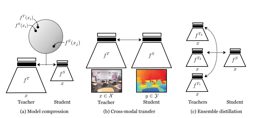
Often we wish to transfer representational knowledge from one neural network to another. Examples include distilling a large network into a smaller one, transferring knowledge from one sensory modality to a second, or ensembling a collection of models into a single estimator. Knowledge distillation, the standard approach to these problems, minimizes the KL divergence between the probabilistic outputs of a teacher and student network. We demonstrate that this objective ignores important structural knowledge of the teacher network. This motivates an alternative objective by which we train a student to capture significantly more information in the teacher’s representation of the data. We formulate this objective as contrastive learning. Experiments demonstrate that our resulting new objective outperforms knowledge distillation on a variety of knowledge transfer tasks, including single model compression, ensemble distillation, and cross-modal transfer. When combined with knowledge distillation, our method sets a state of the art in many transfer tasks, sometimes even outperforming the teacher network.

Knowledge distillation는 분야는 Teacher에 도움을 받아 Student를 학습시키는 분야를 지칭한다. 대표적으로 (1) cromss-modal Transfer (ex) Bert -> Bio Bert), (2) Model compression, (3) ensemble distillation등에서 사용된다.

대부분의 Loss function은 KL divergence로서 teacher와 student의 output(probability)를 서로 비슷하게 학습하나, 해당 논문은 이러한 기본적인 Loss function보다 서로 representation을 비슷하게 만드는 것이 더 결과가 좋았다고 얘기하고 있다.

따라서, 이러한 Loss를 contrastive 하게 학습하는 CRD (CONTRASTIVE REPRESENTATION DISTILLATION) 를 제시하고 위에서 언급한 각각의 예시에서 모두 SOTA의 성능을 보이는 것을 목표로 한다.

Formulation

• \(y^T\): Output of the teacher
• \(y^S\): Outpuut of the student
• \(\psi\): Knowledge distillation (KD) objective function
• \(\phi_i(a,b)\): KL divergence objective function(Cross Entropy, \(-a\log b\))
• \(x \sim p_{data}(x)\): Data
• \(S = f^S(x)\): Student’s representation
• \(T = f^T(x)\): Teacher’s representation

Introduction

Knowledge distillation은 기존에 KL-Divergence를 활용하여 Teacher와 Student의 Output (probability)의 distribution을 비슷하게 학습하였다. 이러한 Loss funciton은 \(\psi(y^S, y^T) = \sum_{i} \phi_i (y_i^S, y_i^T)\)로서 학습할 수 있다.

이러한 KL-Divergence의 문제점으로 논문 저자들은 다음과 같이 얘기하고 있다.

Such a factored objective is insufficient for transferring structural knowledge, i.e. dependencies between output dimensions i and j. This is similar to the situation in image generation where an L2 objective produces blurry results, due to independence assumptions between output dimensions.

(위와 같은 문장은 잘 이해하지 못하였습니다., 예시로 든 L2로서 image를 generation하는 model들은 Sharp하게 나오지 않아 GAN 기반 으로서 학습하는 model이 있습니다.) 즉, 논문 저자들은 단순히 1-dimension(Output probability)만은 관계를 고려하는 것은 문제점이 발생하게 되므로, “higher-order dependencies”의 correlation을 고려할 수 있는 Loss를 제안한다. 해당 Loss는 representational space를 contrasitive loss기반으로서 학습하는 방법이다.

참조. Contrastive learning
Contrasitive Learning에 대하여 생소하신 분들은 해당 논문의 저자가 쓴 Contrastive Multiview Coding을 읽으시면 이해하기 편하십니다.

Method

Method Contrastive Loss

Method 1. Condition
해당 Loss를 설명하기 위하여 다음과 같은 가정에서 진행하였다.
Contrastive Loss를 적용하기 위하여 1개의 positive (Label=1)과 N개의 negative(Label=0)을 선택하는 sampling을 진행 한다.

위와 같은 조건일 때 Sampling에 해당하는 새로운 probability distribution (\(q(\cdot)\))와 prior를 아래와 같이 정의할 수 있다.

• \(q(T,S| C=1) = p(S,T)\): Joint distribution
• \(q(T,S| C=0) = p(S)p(T)\): Marginal distributions
• \(q(C=1) = \frac{1}{N+1}\): Positive sample prior
• \(q(C=0) = \frac{N}{N+1}\): Negative sample prior

위의 수식을 intuitively 하게 생각하면 Positive의 sample에 대하여서는 Student와 Teacher의 representation의 위치가 비슷하게 위치하고, Negative의 sample에 대해서는 독립적이여도 상관없다는 의미이다.

Method 2. Bayes’ rule & Mutual information
위의 수식을 활용하여 Bayes’ rule을 적용하면 아래와 같이 수식을 풀어쓸 수 있다.

$$q(C=1|T,S) = \frac{q(T,S|C=1)q(C=1)}{q(T,S|C=0)q(C=0)+q(x,y|C=1)q(C=1)}$$

$$=\frac{p(T,S)}{p(T,S) + Np(T)p(S)}$$

위의 수식을 Multual information을 사용하게 되면 아래와 같이 쓸 수 있다.

$$\log q(C=1|T,S) = \log \frac{p(T,S)}{p(T,S)+Np(T)p(S)}$$

$$= -\log (1+N \frac{p(T)p(S)}{p(T,S)}) \le -\log (N) + \log \frac{p(T,S)}{p(T)p(S)}$$

위의 식에서 Multuual Information으로서 나타내면 아래와 같이 나타낼 수 있다.

$$\log q(C=1|T,S) + \log (N) \le \log \frac{p(T,S)}{p(T)p(S)}$$

$$\log (N) + \mathbb{E}_{q(T,S|C=1)} \log q(C=1|T,S) \le I(T;S)$$

위의 수식을 살펴보면 Teacher와 Student의 representation의 multual information(\(I(T;S)\))은 Lower bound인 \(\mathbb{E}_{q(T,S|C=1)} \log q(C=1|T,S)\)을 maximize하는 것으로 해결할 수 있다.

Method 3. Latent representation -> 0~1

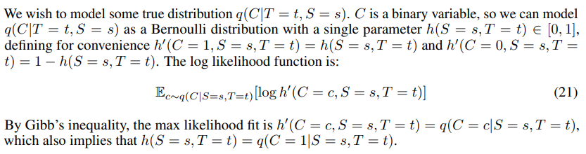
하지만, 현재 문제는 \(q(T,S|C=1)\)의 True distirbution을 알 수 없다는 문제가 발생하게 된다. (\(q(\cdot)\)을 \(p(\cdot)\)에 대한 조건부 확률로 정의하였기 때문에)

논문의 저자는 위와 같은 \(q(T,S|C=1)\)를 대신하기 위하여 sampling한 분포인 \(h: \{T,S\} -> [0,1]\)로서 나타내었다.
즉 True distirubtion을 추정하기 위하여 sampling을 실시한 결과(Input -> Embedding의 값)로 추정하고, 이는 Model을 학습함으로서 점점 정확해 질 것이다. \([0,1]\)의 범위로서 나타내기 위하여 아래와 같이 표현하였다.

$$h(T,S) = \frac{e^{g^T(T)' g^S(S)/\gamma}}{e^{g^T(T)' g^S(S)/\gamma} + \frac{N}{M}}$$

• \(M\): cardinality of the dataset (Training Data개수)
• \(\gamma\): temperature that adjusts the concentration level.
• \(g^S, g^T\): linearly transform them into the same dimension and further nofrmalize them by L-2 norm before the inner product

위의 수식을 살펴보게 되면, 다음과 같다. Goal: Teacher와 Student의 latent representation이 얼마나 관계가 있는지 나타낸다.
Problem: (1) 서로의 Diemsnion이 다르다. (2) 0~1의 값으로 나타내어야 한다.

1. Teacher와 Student의 representation(\(T, S\))를 같은 diemsnion으로 나타내기 위하여 linear transform을 사용하여 옮긴다.
2. 서로 얼마나 관계가 있는지 살펴보기 위하여 dot production를 사용한다.(\(g^T(T)'g^S\))
3. 0~1사이의 값으로 나타내기 위하여 분모에 \(\frac{N}{M}\)을 추가한다.

위의 수식을 살펴보게 되면 다음과 같은 의미를 가지게 된다.

1. Sample의 개수가 많아질 수록 같은 correlation이여도 높은 값을 가진다.
2. Teacher와 Student의 leatent representation이 비슷할수록 높은 값을 가진다.

\(\gamma\)는 hyperparamter로서 나중에 ablation으로서 performance의 변화를 측정한다.

Method 4. \(q(C=1|T,S) -> h: \{T,S\}\)
위에서 정의한 \(h: \{T,S\}\)를 활용하여 Objective funciton을 다시 정의하면 아래와 같다.

$$L_{critic}(h) = \mathbb{E}_{q(T,S|C=1)} \log q(C=1|T,S)$$

$$= \mathbb{E}_{q(T,S|C=1)}[\log h(T,S)] + N \mathbb{E}_{q(T,S|C=0)} [1-\log(h(T,S))]$$

$$h^* = \text{argmax}_h L_{critic}(h) - (1)$$

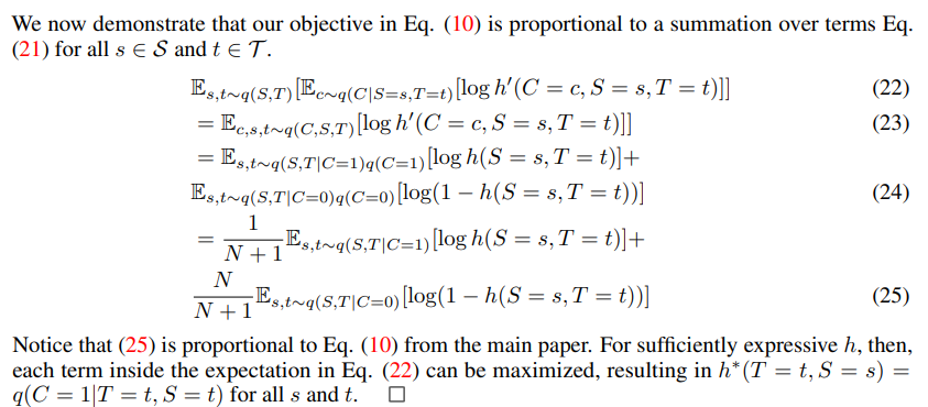
위에서 정의한 (1)의 식을 Multual information에 적용하면 다음과 같다. (Appendix Proof that \(h^*(T,S) = q(C=1|T,S)\) 참조)

$$I(T;S) \ge \log (N) + \mathbb{E}_{q(T,S|C=1)} [\log h^* (T,S)]$$

위의 수식에서 Lower bound를 높이기 위해서는 $\log h^* (T,S)$ 의 값을 높여야 하며, 이는 Student Model을 학습하여야 한다. (Teacher는 학습하였고 고정되었다고 가정.)

$$f^{S*} = \text{argmax}_{f^S} \mathbb{E}_{q(T,S|C=1)} [\log h^* (T,S)] - (2)$$

(1)과 (2)의 수식을 활용하여 최종적인 Objective Funciton을 나타내면 아래와 같다.

$$f^{S*} = \text{argmax}_{f^S} \text{max}_h L_{critic}(h)$$

$$=\text{argmax}_{f^S} \text{max}_h \mathbb{E}_{q(T,S|C=1)} [\log h (T,S)] + N \mathbb{E}_{q(T,S|C=1)} [\log (1-h (T,S)) ]$$

위의 수식에 대하여 논문 저자는 다음과 같이 표현하고 있다.

which demonstrates that we may jointly optimize \(f^{S}\) at the same time as we learn \(h\). We note that due to (16), \(f^{S*} = \text{argmax}_{f^S}L_{critic}(h)\), for any \(h\), also is a representation that optimizes a lower-bound (a weaker one) on mutual information, so our formulation does not rely on \(h\) being optimized perfectly

(정확히 이해하지 못하였습니다.) 우리는 두개의 \(f^{S}, h\)를 학습하여야 되며, 이는 동시에 이루워질 수 있다. Intuitively하게 생각하면, h는 Embedding -> 0~1로 mapping하는 하나의 Layer로서 생각해보자. 그렇다면 우리는 Input -> \(f^{S}\) -> \(h\)의 Architecture모델로 생각할 수 있고, 같이 학습할 수 있다. 왜냐하면 h와 상관없이 \(T, S\)의 값이 서로 비슷한 것 만으로도 Mutual information의 Lower bound를 올릴수 있기 때문이다.

위의 내용을 정리하면 아래와 같다.

1. “Higher-order dependencies”의 correlation을 고려하기 위하여 Teacher와 Student의 Latent representation간의 Multual information을 최대화 한다.
2. “Mutual information”의 수식은 \(\log (N) + \mathbb{E}_{q(T,S|C=1)} \log q(C=1|T,S) \le I(T;S)\)으로서 Lower bound를 maximize한다.
3. \(q(C=1|T,S)\)의 True distirbution을 알 수 없으므로 sampling한 분포인 \(h: \{T,S\} -> [0,1]\) 로서 표현한다.
4. 최종적으로 Lower bound를 maximize하기 위하여 Student model또한 학습되어야 한다.\(f^{S*} = \text{argmax}_{f^S} \mathbb{E}_{q(T,S|C=1)} [\log h^* (T,S)]\)

Appendix. Memory buffer for implementation
위의 Objective Function을 수행하기 위해서는 Positive Sample과 Negative Sample이 필요하게 된다. 여기서 문제점은 만약 Batch Size=256이고, 각 Positive Sample마다 Negative sample이 1000개로서 Setting하게 되면, 256 * 1000개의 Sample이 필요하게 된다. 이러한 문제점은 Out-of-memory를 발생시키게 되므로, memory buffer를 만들어서 이러한 문제를 해결하였다. (Contrastive learning에서 많이 사용하는 방식이다.)

Appendix. Mutual information
Multual information는 확률변수 X와 Y의 상호의존성을 엔트로피를 이용해 정량화한 형태로서 아래와 같이 나타낼 수 있다.

$$I(X;Y) = \sum_{i=1}^N \sum_{j=1}^M p(x_i, y_j) \log \frac{pp(x_i, y_i)}{p(x_i)pp(y_j)}$$

$$I(X;Y) = H(X) + H(Y) - H(X,Y)- (1)$$

$$= H(X) - H(X|Y)- (2)$$

$$= H(Y) - H(Y|X)- (3)$$

$$(H(X|Y) = -\sum({j=1}^M p(y_j) \sum_{i=1}^N p(x_i|y_i) \log p(x_i|y_j))$$

(1) 확률변수 X, Y가 독립일 경우보다 얼마나 불확실성이 감소하였는가
(2) 확률변수 X의 불확실성이 Y를 아는 것으로 인해 얼마나 감소하였는가
(3) 확률변수 Y의 불확실성이 X를 아는 것으로 인해 얼마나 감소하였는가

참조: mons1220 Blog

Appendix Proof that \(h^*(T,S) = q(C=1|T,S)\)

Experiments

Dataset

1. CIFAR-100
2. ImageNet
3. STL-10
4. TinyImageNet
5. NYU-Depth V2

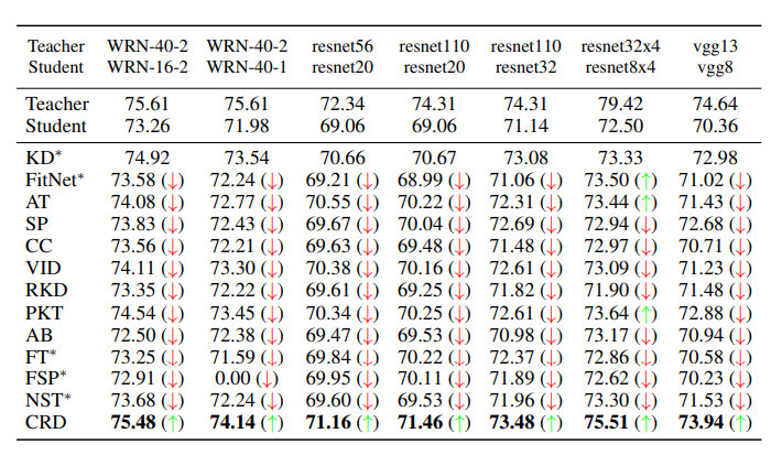
Model compression
CIFAR-100 Dataset을 사용하여 Model Compression성능을 측정하였고, 아래의 Table과 같이 기존에 많이 사용하던 KD보다 성능이 향상된 것을 알 수 있다.

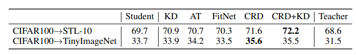
CROSS-MODAL TRANSFER
Cross-Modal transfer를 진행하였고, CRD or CRD+KD가 다른 Method들에 비하여 Outperform을 보여주었다.