Paper01. DANN:Cross-Cell-Type Prediction of TF-Binding Site by Integrating Convolutional Neural Network and Adversarial Network

Cross-Cell-Type Prediction of TF-Binding Site by Integrating Convolutional Neural Network and Adversarial Network

https://www.ncbi.nlm.nih.gov/pmc/articles/PMC6679139/pdf/ijms-20-03425.pdf

Abstract
Transcription factor binding sites(TFBs)는 gene expression regularization을 담당하는 매우 중요한 역할이 있다.
이러한 TFBs를 찾기위한 많은 Model들은 많은 Dataset이 필요로 한다.

하지만, 이러한 Dataset은 많지 않은게 현재 사실이며, 해당 논문에서 제시하는 DANN_TF는 이러한 부족한 Label을 Prediction하는 Model이며 크게 1) Feature Extractor(CNN), 2) Label Predictor, 3) Domain Classifier, 1,3은 Adversial Network로서 구성된다.

Adversial Network라고 불리는 이유는 Corss Cell Types에서 CNN으로서 공통된 Feature를 Extraction하나, Domatin Classifier에서는 이러한 공통된 Feature로서 어떤 Cell Type인지 Classifier하기 때문이다. 즉, GAN에 적용하여 생각하면 Feature Extractor가 어떤 Cell Type인지 판단못하게 공통된 Feature를 추축하게 되면, Domain Calssifier에서 Discriminator의 역할을 수행하는 것 이다.

25 cell-type TF pairs(5 Cell Type * 5 TF)로서 Feature Extractor가 Trainning되고, 총 65 cell-type TF pairs(5 Cell Type * 13 TF)로서 전체적인 Network가 Trainning된다. => 최종적인 AUC는 96.9%이다.

많은 Studies에서 Cell Types이 달라도 TF는 Common histone motifications와 common binding motifs를 가지고 있다는 것이 밝혀졌다.

따라서 이러한 특성을 사용하게 되면, Different Cell Types여도 TFBs를 Prediction할 수 있다는 것 이다.

참고
기존에 배웠던 DeepSea, DanQ에 대해서도 언급하고 있다. 휼륭한 Model이지만, 해당 Paper에서 강조하는 것은, 이러한 Model을 Trainning하기 위한 Dataset은 Label이 없는 경우가 많아서 구축하기 힘들다. => 따라서, Dataset을 많이 확보하기 위하여 서로다른 Cell Types를 가져와 사용할 것 이며 -> Common histone motification, binding motifs가 있으므로 Cell Type과 상관없이 TFBs를 Prediction할 수 있다. -> Dataset의 Label을 서로 보완하면서 Dataset을 구축할 수 있다.

DANN

먼저 Paper에서 사용하는 Model인 DANN(Domain-Adversarial Trainning of Neural Network)의 구조부터 살펴보면 다음과 같다.

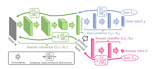
Model을 크게 2개의 Network로서 생각하면 다음과 같다.

• Feature Extractor + Label Predictor: Classification Model
• Feature Extractor + Domain Classifier: GAN

대표적인 2개의 Model로서 표현하면 위의 구조와 같다.
Classification Model은 Input Sequence에 따라 TFBS or non-TFBS인지 Classification하는 Model이다.
GAN Model은 Input Sequence에 따라 어느 Cell Type인지 Domain을 Classification하는 Model이다.

즉, DANN은 Classification Model + GAN Model인 Model인 것 이다. 이러한 Model은 크게 다시 3개의 Sub Network를 구별하면 다음과 같다.

• Feature Extractor: Domain에 상관없이 Common한 Feature를 Extraction하는 역할
• Label Predictor: Common한 Feature로서 Label을 Classification하는 역할
• Domain Classifier: Common한 Fuature로서 Domain을 Classification하는 역할

GAN으로서 생각하면 간단하다. Feature Extractor는 Domain에 상관없이 Common한 Feature를 뽑게 되지만, Discriminator역할을 하는 Domain Classifier에서 어느 Domain인지 판단하게 되면, Common한 Feature에는 Domain에 대한 Feature가 포함되있다는 것을 알 수 있다.
이러한 Common Feature의 Domain Information를 없게하기 위하여 Gradient Reversal Layer를 통하여 Gradient를 반대로 Backpropagation을 수행하게 되면, Feature Extractor는 weight가 Update되면서, Domain에 대한 정보는 점점 사라지고 Common한 Feature를 Extraction하도록 Update될 것 이다.
이러한 결과로서 Featire Extractor는 Domain에 대한 Information이 없어진 Domaain Independent Feature를 Extraction하게 될 것이고, Domain Classifier는 어느 Domain인지 Classification하기 어려워질 것 이다.

결과적으로 기존의 Feature Extractor + Label Predictor의 Model에서 Feature Extractor와 Adversial Network인 Domain Classifier를 추가함으로서 Cross Cell Type에 대한 TFBs를 Classification할 수 있는 Model이 되는 것 이다.

Classificaiton Model은 많이 다뤘으니, 이번 DANN이 다른 Model과 다른 GAN을 추가하여 어떤 효과를 얻는지, 이로 인하여 어떻게 Model이 Update되는지 알아보자.

Damain Adaptation
먼저 Model의 General한 Formula를 살펴보기 위하여 문제를 단순화 해보자.

• Source Domain: \(D_S\) => 현재 Label을 알고있는 Domain
• Target Domain: \(D_T\) => Label을 모르는 Domain
• \(n\): Num of Source Domain Dataset
• \(n^{'}\): Num of Target Domain Dataset
• \(N = n+n^{'}\): Total Num of Dataset

위와 같이 단순히 2개의 Domain만 존재하고, 한개의 Domain에 대해서만 Label을 알고 있다고 가정하면 Dataset에 대하여 다음과 같이 나타낼 수 있다.

$$S = \begin{Bmatrix} (x_i,y_i) \end{Bmatrix}_{i=1}^{n} \sim^{iid} (D_S)^n$$

$$T = \begin{Bmatrix} (x_i) \end{Bmatrix}_{i=n+1}^{N} \sim^{iid} (D_T^{X})^{n^{'}}$$

일반적인 ML과 같다는 것을 파악할 수 있을 것이다. Train Dataset(\(D_S^{X}\))으로서 Model을 Update시키고, Test Dataset(\(D_T^{X}\))에서 Model의 Prediction이 실제와 같도록 Update시키는 것과 같도록 하는 것을 알 수 있다. Classifier가 \(\eta: X \rightarrow Y\)라고 한다면 식은 다음과 같을 것 이다.

$$R_{D_{T}}(\eta) = Pr_{(x,y) \sim D_T} (\eta(x) \neq y)$$

위과 같은 Risk \(R_{D_{T}}(\eta)\)가 최소화 되도록 Model을 Update하게 하는 것 이다.

Domain Divergence
위와 같은 문제를 해결하기 위하여 KL Divergence와 같은 개념인 Domain Divergence를 사용하게 된다.

즉, 최종적인 Model의 Loss는 Label Predictor Loss(= Source Classification Error) + Domain Classifier( = Domain Divergence)으로 정의될 것인데, 여기서 Domain Classifier의 Loss를 Domain Divergence로서 표시한다는 것 이다.

2Domain간의 Districution을 비교하는 Domain Divergence로서는 \(\mathcal{H}\)-divergence가 사용되고 식으로서 표현하면 다음과 같다. (Binary Classifier라는 가정이 필요하다. 즉, 이 Domain이 맞는지 맞지 않는지 표현하는 것 이다.)

Defination 1(Kifer et al., 2004)

$$d_{\mathcal{H}}(D_{S}^{X},D_{T}^{X}) = 2 sup_{\eta \in \mathcal{H}} |Pr_{x \sim D_{S}^{X}}[\eta(x)=1]-Pr_{x \sim D_{T}^{X}}[\eta(x)=1]|$$

$$\mathcal{H}: \text{Hypothesis Class}$$

위의 수식에 값을 대입하여 보자. 극단적인 예를 살펴보면 다음과 같다.

• 둘다 Class Label을 1로서 Prediction => 0: 어느 Domain인지 구별하지 못한다.
• Label Class Label 1, Target Class Label 0 => 1: 어느 Domain인지 확실히 구별한다.
• 둘다 Class Label을 0으로서 Prediction => 0: 어느 Domain인지 구별하지 못한다.

또한 한가지 더 고려해야 할 점은, \(\mathcal{H}\)의 차원이 커질수록 Loss가 0이되는 Optimal한 Minumum을 찾을 수 있지만, 결국 ML의 고질적인 문제처럼 Dimension이 커짐 => Complexity가 커짐 => Overfitting의 위험 발생 이라는 결론이 다다르게 된다.
따라서, \(\mathcal{H}\)은 주어진 Dimension에서 Approximation하면서 Grid하게 Search해나가는 방향으로 바꿔야 한다는 것을 알 수 있다.

Defination 2(Ben-David et al., 2006, 2010)

$$\hat{d_{\mathcal{H}}}(S,T) = 2 (1-min_{\eta \in \mathcal{H}} [\frac{1}{n}\sum_{i=1}^{n} I[\eta(x_i)=1] + \frac{1}{n^{'}}\sum_{i=n+1}^{N}I[\eta(x_i)=0]])$$

$$\mathcal{H}: \text{Hypothesis Class & Symmentric}$$

$$I[\alpha]: \text{Indicator function which is 1 if predicate } \alpha \text{ is ture, and 0 otherwise}$$

위의 식을 좀 더 쉽게 표현하기 위하여 근사적으로 표현한 PAD(Proxy A Distance)로서 표현하면 다음과 같다.

$$\hat{d}_{A} = 2(1-2\epsilon)$$

위의 식에서 \(min_{\eta \in \mathcal{H}} [\frac{1}{n}\sum_{i=1}^{n} I[\eta(x_i)=1] + \frac{1}{n^{'}}\sum_{i=n+1}^{N}I[\eta(x_i)=0]])\)을 자세히 살펴보게 되면, Model이 Source Domain인지 Target Domain인지 Classification하는 문제라고 생각할 수 있다. 즉, PAD에서 \(\epsilon\)으로서 표현한 것은 Classificaiton의 Error라고 표현할 수 있다는 것 이다.

Defination 3(Ben-David et al., 2006, 2010)
Generalization하기 전에 수식들을 유도한 것은 다음과 같다.
최종적인 목적은 \(R_{D_{T}}(\eta)\)를 최소화 하는 것 이다.
위의 Error는 1. Classification Error(Label이 있는 Source Data의 Classification Error) + 2. Domain Classification Error(Label이 있는 Source Data와 Label이 없는 Target Data의 Classification의 Error)로서 표현된다.
Domain Classification의 Error는 두 Districution이 비슷하게 만들면, Domain Classifier는 판별하지 못할 것 이고 이러한 방법으로서 \(\mathcal{H}\)-divergence으로서 구하게 된다.

\(\mathcal{H}\)-divergence을 구하는 방법은 Defination1에서 정의하였으나 \(\mathcal{H}\)의 Complexity를 고려하기 어렵다. 따라서 Defination 2에서 PAD로서 식을 간소화 하고 Model의 Complexity를 고려한 식으로서 변경한다.

\(\mathcal{H}\)-divergence는 따라서 Defination 2식과 Model의 Complexity를 고려한 식의 Upper bound로서 표현할 수 있게 되어 최종적인 Loss는 다음과 같이 표현할 수 있다.(A theory of learning from different domains[2]에서 \(\mathcal{H}\)-divergence가 Divergence + constant Complexity Term으로서 Upper Bound가 되는 것을 밝혔다.)

위의 Condidtion을 모두 고려하여 General한 Formula를 표현하면 다음과 같다. (해당 식은 VC Dimension으로서 Model의 Complexity를 계산한 수식이라고 한다. VC Dimension에 대해서는 좀 더 공부하기로 한다.)

$$\begin{align} R_{\mathbb{D}_T}(\eta) \leq &R_{S}(\eta) + \sqrt{\frac{4}{m}(d\log\frac{2em}{d}+\log\frac{4}{\delta})}\\ &+ \hat{d}_{\mathcal{H}}(S,T) + 4 \sqrt{\frac{1}{m}( d\log\frac{2m}{d}+\log{4}{\delta})}+ \beta, \end{align}$$

$$\beta \geq \inf_{\eta^*\in\mathcal{H}}\left[ R_{\mathbb{D}_S}(\eta^*) + R_{\mathbb{D}_T}(\eta^*) \right]$$

$$R_{S}(\eta) = \frac{1}{m}\sum_{i=1}^m I\left[ \eta(x_i) \neq y_i \right]$$

최종적인 식은 어렵지만 간단하게 표현하면 다음과 같다.

1. \(R_{\mathbb{D}_T}(\eta)\)을 Minimize하기 위해서는 Upper Bound를 Minimize하는 문제로 Approximation하게 바꿀 수 있다.

2. UpperBound의 Formula를 Minimize하는 문제는 다음과 같이 나눌 수 있다.
   • \(R_{S}(\eta)\) Minimize: Label이 있는 Source Domain에서 Classification을 잘 할수있도록 Loss를 Minimize - (1)
   • \(\hat{d}_{\mathcal{H}}(S,T)\) Minimize: Source Domain과 Target Domain을 Domain Classifier에서 잘 구별하지 못하도록 Update - (2)
   • \(\sqrt{\frac{4}{m}(d\log\frac{2em}{d}+\log\frac{4}{\delta})}+4 \sqrt{\frac{1}{m}( d\log\frac{2m}{d}+\log{4}{\delta})}+ \beta\): Model의 Complexity를 측정 - (3)
3. (2)의 Loss를 줄이기 위하여 Model의 Complexity를 증가시키면, (3)의 값도 증가하게 되어 전체적인 Upper Bound의 값이 증가하게 된다. => 적절한 Complexity를 선택하여야 한다.

DANN Model

위에서 어떻게 DANN이라는 Model을 Update시키는지에 대하여 General한 Model에 대하여 알아보았다.
이제 실제 Paper의 Model에서 어떻게 Model을 구성하고 Udpate하는지 알아보면 다음과 같다.

먼저, Paper에서 제공하는 Model을 살펴보면 다음과 같다.

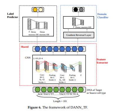
DeepSea와 비교하게 되면, DeepSea의 경우에는 Output으로서 919개의 Chromatin Feature를 뽑아내게 된다. 각각의 Cell Type과 DHS, TF binding, Histone mark에 대하여 뽑아내게 된다. 해당 Paper에서는 Domain Classifier를 추가시킨 DANN Model로서 이러한 Cell Type을 각각 적용시키지 않고 Cross Cell Type에 해당되는 Model을 만들 수 있는 것 이다.

각각의 3개의 Sub Network(Feature Extractor, Label Predictor, Domain Classifier)로서 나누어서 생각하면 다음과 같다.

Feature Extractor

• Convolution Layer: \(Y_{i,k} = conv_{i,k}(X) = ReLU(\sum_{m=0}^{M-1} \sum_{n=0}^{N-1} W_{mn}^{k} X_{i+m,n})\)
• Poolying Layer: \(pooling_{i,k}(Y) = max(Y_{ixM,k},Y_{ixM+1,k},...,Y_{ixM+M-1,k})\)
• Output: \(Z = pooling(conv(pooling(conv(X))))\)

위의 식을 살펴보게 되면, 일반적인 CNN의 Model로서 Input에 대하여 Convolution -> Activation Function(ReLU) -> Pooling(Max Pooling)으로서 Output인 Z를 생성하는 것을 알 수 있다.

Label Predictor

$$G_{l}(Z) = softmax(FC(FC(Z)))$$

일반적인 CNN의 Output Layer로서 CNN Feature Extractor로 뽑은 Feature Z를 Input으로 받아 FC Layer를 거치고 Softmax를 통하여 Output을 뽑아내는 것을 확인할 수 있다.

Domain Classifier

$$G_{d}(Z) = softmax(relu(FC(Z)))$$

Label Predictor와 마찬가지로 CNN Feature Extractor로 뽑은 Feature Z를 Input으로 받아 FC Layer를 거치고 Softmax를 통하여 Output을 뽑아내는 것을 알 수 있다. (Source Domain or Target Domain Classification)

Object Function
위에서 최종적인 Loss는 총 3가지의 Loss합으로서 이루워지는 것을 확인하였다.
(3)의 경우에는 ML의 Weight regularization, Dropout, Early Stopping등의 기법으로 어느정도 해결되기 때문에 (1), (2)를 고려하여 Model의 LossFunction을 구성해야 된다는 것을 알 수 있다.

1. Label Predictor Loss

$$R_{S}(\eta)$$

Classification의 Loss같은 경우 일반적으로 구성하는 Loss와 똑같이 구성하면 된다.

2. Domain Classifier Loss

$$\hat{d_{\mathcal{H}}}(S,T) = 2 (1-min_{\eta \in \mathcal{H}} [\frac{1}{n}\sum_{i=1}^{n} I[\eta(x_i)=1] + \frac{1}{n^{'}}\sum_{i=n+1}^{N}I[\eta(x_i)=0]])$$

기본적으로 LossFunction을 CrossEntropy로 구성하여서 Domain Classifier를 잘 역할을 하도록 Loss를 적용할 수 있다.
중요한 것은 이 Domain Classifier Loss를 Feature Extractor에 어떻게 전달하는 지가 중요하다. Feature Extractor에 전달되는 Loss는 위에 Loss처럼 Domain에 Indepedent한 Feature를 뽑기 위하여 Domain에 관한 Loss가 전해져서 Domain을 잘 구별하는 것이 아닌 반대로의 Loss가 Backpropagation으로서 전달되어야 할 것 이다. 따라서 Paper에서는 이러한 Gradient의 부호를 바꾸는 Layer로서 GRL(Gradient Reversal Layer)를 추가하였다.

최종적인 Loss를 정의하면 다음과 같다.

• \(G_f: \text{Feature Extractor, }G_y: \text{Label Predictor, }G_d: \text{Domain Classifier }\)
• \(\theta_f: \text{Feature Extractor Weight, }\theta_y: \text{Label Predictor Weight, }\theta_d: \text{Domain Classifier Weight }\)
• \(L_y: \text{Label Predictor Loss, }L_d: \text{Domain Classifier Loss }\)
• \(\hat{\theta_f},\hat{\theta_y},\hat{\theta_d}\): Saddle Point

$$E(\theta_f,\theta_y,\theta_d)=\frac{1}{n}\sum_{i=1}^n\mathcal{L}^i_y(\theta_f,\theta_y)-\lambda\left( \frac{1}{n}\sum_{i=1}^n\mathcal{L}^i_d(\theta_f,\theta_d) + \frac{1}{n'}\sum_{i=n+1}^N\mathcal{L}^i_d(\theta_f,\theta_d) \right)$$

$$\begin{align} &(\hat{\theta_f}, \hat{\theta_y}) = \underset{\theta_f,\theta_y}{arg\min} ~E(\theta_f,\theta_y,\hat{\theta_d}), \\ &\hat{\theta_d}= \underset{\theta_d}{arg\max} ~E(\hat{\theta_f},\hat{\theta_y},\theta_d). \end{align}$$

위와같은 Loss를 정의하였다면, Weight Update는 다음과 같이 이루워진다.(u=learning rate)

$$\theta_f \leftarrow \theta_f -u(\frac{\partial L_y^i}{\partial \theta_f} -\lambda \frac{\partial L_d^i}{\partial \theta_f})$$

$$\theta_y \leftarrow \theta_y -u\frac{\partial L_y^i}{\partial \theta_y}$$

$$\theta_d \leftarrow \theta_d -u\lambda \frac{\partial L_d^i}{\partial \theta_d}$$

$$\lambda= \begin{cases} 1, & \mbox{when }\theta_d \mbox{ update} \\ \frac{2}{1+exp(-10p)}-1, & \mbox{when } \theta_f \mbox{ update, p is 0 to 1 linearly change} \end{cases}$$

최종적인 위의 식을 살펴보게 되면, DomainClassifier의 Loss가 Feature Extractor에 갈때는 Loss의 부호가 반대가 되는 것을 확인할 수 있다. 또한 \(\lambda\)값을 0~1로서 Smooth하게 올리는 이유에 관해서는 정확한 설명이 없으나, TFBs를 어느정도 Prediction할 수 있는 상황에서 => Feature를 어느정도 뽑을 수 있는 상황에서 Domain에 상관없는 Domain Independent Feature를 뽑게할 수 있도록 기대할 수 있다.

참고: GRL(Gradient Reversal Layer)
Domain Classifier -> Feature Extractor로 넘어갈때 Loss의 부호를 바꾸기 위하여 GRL을 사용한다. 단순히 -1을 곱하는 것은 각각의 Gradient를 고려하는 것이 아닌, 모든 Summation혹은, 계산된 값에 부호를 붙이는 것 이기 때문이다.

따라서 해당 논문은 Forward, Backward에 대하여 다음과 같이 표현하고 있다.

• \(R(x) = x\): Forward
• \(\frac{dR}{dx} = -I\): Backward, I:identity matrix

Experiment

Trainning시키기 위한 Dataset의 구조는 다음과 같다.

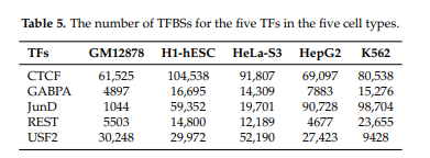
5개의 Cell Types와 5개의 Transcription Factor로서 25 Cell-Type TF pairs에 대하여 Trainning을 하게 된다.

Paper는 Adversial Netowrk를 추가한 DANN_TF를 비교하기 위하여 Domain Classifier가 없는 Base Line과의 성능비교를 계속하여 하고 있다. 각각의 자세한 Model은 다음과 같다.

• BaseLine Model: Feature Extractor + Label Predictor로서 Adversial Network가 없는 Model
• DANN-TF: Featrue Extractor + Label Predictor + Domain Classifier

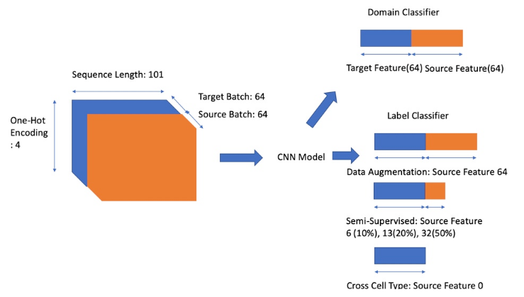
Mdel의 구조부터 살펴보면 다음과 같다.

• Input: 101(Length)x4(One-Hot Encoding)x128(Batch)
• Batch: 128
• Source: 64
• Target: 64
• Label Predictor: TF or Not TF
• Doain Classifier: Source Domain or Target Domain

위와 같은 동일한 Experiment를 Setting하고 다음과 같이 크게 3가지로 나누어서 Experiment를 실시하였다.

• 2.4. Result of Data Augmentation by DANN_TF
• 2.5. Results of Semi-Supervised Prediction by DANN_TF
• 2.6. Results of Cross-Cell-Type Prediction by DANN_TF

각각의 Experiment의 기준은 Target Data의 Label여부 정도로서 Model의 성능을 평가하였다.
각각의 Target Data의 Label 여부는 다음과 같다.

• 2.4: 100%
• 2.5: 10%, 20%, 50%
• 2.6: 0%

이러한 Experiment를 구성하기 위하여 DANN의 Model을 생각하면 다음과 같다.

실제 Code에서 살펴보면 다음과 같다.

# Train
    if supervise == 0:
        sup_flag = 64
    elif supervise == 1:
        sup_flag == 70
    elif supervise == 2:
        sup_flag == 77
    elif supervise == 5:
        sup_flag == 96
    else:
        sup_flag = 128

# Model
source_features = tf.slice(self.feature, [0, 0], [sup,-1])
classify_feats = tf.cond(self.train,lambda: source_features, lambda:all_features)

all_labels = self.y
# source_labels=all_labels
source_labels = tf.slice(self.y, [0, 0], [sup,-1])

위와 같은 실험의 Metric으로서는 AUC, F1 Score로서 각각 BaseLine과 DANN_TF의 Model을 평가하게 된다. 또한 Sampling의 효과를 없애기 위하여 CrossValidation을 실행하게 됩니다.

Model

__init__

    def __init__(self,embedding_size,sequence_length,label_classes,domain_classes,
                 filter_height,filter_width,num_filters_1,num_filters_2,hidden_dim, sup):

        self.X = tf.placeholder(tf.float32, [None, embedding_size, sequence_length, 1])
        self.y = tf.placeholder(tf.float32, [None, label_classes])
        self.domain = tf.placeholder(tf.int32, [None, domain_classes])
        self.l = tf.placeholder(tf.float32, [])
        self.train = tf.placeholder(tf.bool)
        self.flip_gradient = FlipGradientBuilder()

        X_input=self.X

위의 Code를 살펴보게 되면, Data X,Y와 Domain에 대한 정보 domain을 정의하는 것을 알 수 있습니다.
None의 경우에는 Batch Size에 맞추기 위하여 None으로서 정의하였습니다.

• embedding_size: 4 => One-Hot-Encoding
• sequence_length: 101 => Sequence Length
• label_classes: 2 => TF or Not
• domain_classes: 2 => Source or Target

각각의 Argument는 위와 같은 의미를 가지고 있습니다.

Feature Extractor

        with tf.variable_scope('feature_extractor'):
            W_conv0 = weight_variable([filter_height, filter_width,1, num_filters_1])
            b_conv0 = bias_variable([num_filters_1])
            h_conv0 = tf.nn.relu(conv2d(X_input, W_conv0) + b_conv0)

            #ksize: [batch,height,wide,in_channel], generally batch=1,channel=1
            # strides :[batch,height,wide,in_channel],generally batch=1,channel=1
            h_pool0=tf.nn.max_pool(h_conv0, ksize=[1, 1, 5, 1],
                           strides=[1, 1, 2, 1], padding='SAME')


            W_conv1 = weight_variable([filter_height, filter_width, num_filters_1, num_filters_2])
            b_conv1 = bias_variable([num_filters_2])
            h_conv1 = tf.nn.relu(conv2d(h_pool0, W_conv1) + b_conv1)
            h_pool1 = tf.nn.max_pool(h_conv1, ksize=[1, 1, 5, 1],
                           strides=[1, 1, 2, 1], padding='SAME')
            print("self.h_pool1+++++", h_pool1.shape)
            # The domain-invariant feature
            self.feature = tf.reshape(h_pool1, [-1, 4 * 26 * 48])

            print("self.feature+++++",self.feature.shape)

각각 들어오는 Parameter는 다음과 같습니다.

• num_filters_1 = 32
• num_filters_2 = 48
• filter_height = 4
• filter_width = 5

따라서 계산은 다음과 같습니다.(Convolution같은 경우 Utils에서 padding을 same으로서 조건을 주었습니다.)

• Convolution 0
  • X_input: [128,4,101,1]
  • h_conv0: [128,4,101,32(num_filters_1)] => because of padding same
  • h_pool0: [128,4,51,32(num_filters_1)] => round(101/2) = 51
• Convolution 1
  • h_conv1: [128,4,51,48(num_filters_2)]
  • h_pool2: [128,4,26,48(num_filters_2)] => round(51/2) = 26
• Feature: [128,4 x 26 x 48]

Label Predictor

# MLP for class prediction
        with tf.variable_scope('label_predictor'):
            # Switches to route target examples (second half of batch) differently
            # depending on train or test mode.
            all_features = self.feature
            print("all_featuresall_features",all_features.shape)
            print("self.trainvself.train",self.train)

            source_features = tf.slice(self.feature, [0, 0], [sup,-1])
            classify_feats = tf.cond(self.train,lambda: source_features, lambda:all_features)

            all_labels = self.y
            # source_labels=all_labels
            source_labels = tf.slice(self.y, [0, 0], [sup,-1])

            self.classify_labels = tf.cond(self.train, lambda:source_labels,lambda: all_labels)

            W_fc0 = weight_variable([4 * 26 * 48, hidden_dim])
            b_fc0 = bias_variable([hidden_dim])
            h_fc0 = tf.nn.relu(tf.matmul(classify_feats, W_fc0) + b_fc0)

            W_fc1 = weight_variable([hidden_dim, hidden_dim])
            b_fc1 = bias_variable([hidden_dim])
            h_fc1 = tf.nn.relu(tf.matmul(h_fc0, W_fc1) + b_fc1)


            W_fc2 = weight_variable([hidden_dim, label_classes])
            b_fc2 = bias_variable([label_classes])
            logits = tf.matmul(h_fc1, W_fc2) + b_fc2

            self.pred = tf.nn.softmax(logits)
            print("self.logits+++++", logits.shape)
            print("self.self.classify_labels+++++", self.classify_labels.shape)
            self.pred_loss = tf.nn.softmax_cross_entropy_with_logits(logits=logits, labels=self.classify_labels)

각각 들어오는 Parameter는 다음과 같습니다.

• hidden_dim = 100
• FullyConnected Layer0
• h_fc0: [?,100]: Experiment에 따라서 Target Label의 사용할 Data의 개수를 정한다.
• FullyConnected Layer1
• h_fc1: [?,100]
• FullyConnected Layer2
• logits: [?,2]: TF or TF Not을 Softmax로서 표현하기 위하여 2차원으로서 Prediction한다.

Domain Predictor

# Small MLP for domain prediction with adversarial loss
        with tf.variable_scope('domain_predictor'):
            # Flip the gradient when backpropagating through this operation
            feat = self.flip_gradient(self.feature, self.l)

            d_W_fc0 = weight_variable([4 * 26 * 48, hidden_dim])
            d_b_fc0 = bias_variable([hidden_dim])
            d_h_fc0 = tf.nn.relu(tf.matmul(feat, d_W_fc0) + d_b_fc0)

            d_W_fc1 = weight_variable([hidden_dim, domain_classes])
            d_b_fc1 = bias_variable([domain_classes])
            d_logits = tf.matmul(d_h_fc0, d_W_fc1) + d_b_fc1
            print("self.d_logits+++++", d_logits.shape)
            self.domain_pred = tf.nn.softmax(d_logits)
            self.domain_loss = tf.nn.softmax_cross_entropy_with_logits(logits=d_logits, labels=self.domain)

Domain Classifier도 Label Predictor와 마찬가지로 Source Domin or Target Domain에 따라서 Softmax로서 출력하기 때문에 2차원으로서 Prediction한다.

중요한 것은 Gradient에 대하여 l(위의 논문에서 \(\lambda\))를 곱하여 Gradient Reverse Layer를 거친다는 것 이다.

FilpGradientBuilder

class FlipGradientBuilder(object):
    def __init__(self):
        self.num_calls = 0

    def __call__(self, x, l=1.0):
        grad_name = "FlipGradient%d" % self.num_calls

        @ops.RegisterGradient(grad_name)
        def _flip_gradients(op, grad):
            return [tf.negative(grad) * l]

        g = tf.get_default_graph()
        with g.gradient_override_map({"Identity": grad_name}):
            y = tf.identity(x)

        self.num_calls += 1
        return y

위의 Code를 보게 되면, Forward로 불렀을 경우 아무런 변화는 없으나, Back Propagation(@ops.RegisterGradient(grad_name))에서는 Gradient를 반대로서 전달하는 것을 확인할 수 있다.

참조: Customize Gradient Tensorflow Site

Result

2.4. Results of Data Augmentation by DANN_TF

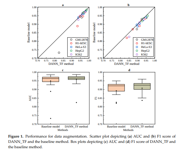
BaseLine과 DANN_TF를 비교하였을 때의 결과는 현재, BaseLine에 비하여 DANN_TF의 Model이 성능이 좋다는 것을 알 수 있다. 25 Cell-type pairs에서 21 pairs가 더 우수하다는 것을 알 수 있다.
평균적으로 AUC는 9.19%, F1 Score는 0.95%정도 향상되었다.

2.5. Results of Semi-Supervised Prediction by DANN_TF

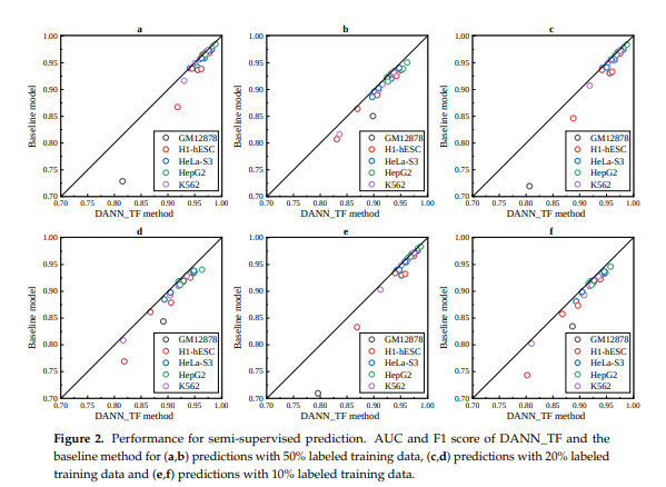
• a,b: Label 50% => AUC, F1
• c,d: Label 20% => AUC, F1
• e,f: Label 10% => AUC, F1

BaseLine보다 DANN_TF가 성능이 좋다는 것을 알 수 있고, 또한 Target Cell에 대하여 Label이 많을 수록 성능이 더 좋아진다는 것을 알 수 있다.

2.6. Results of Cross-Cell-Type Prediction by DANN_TF

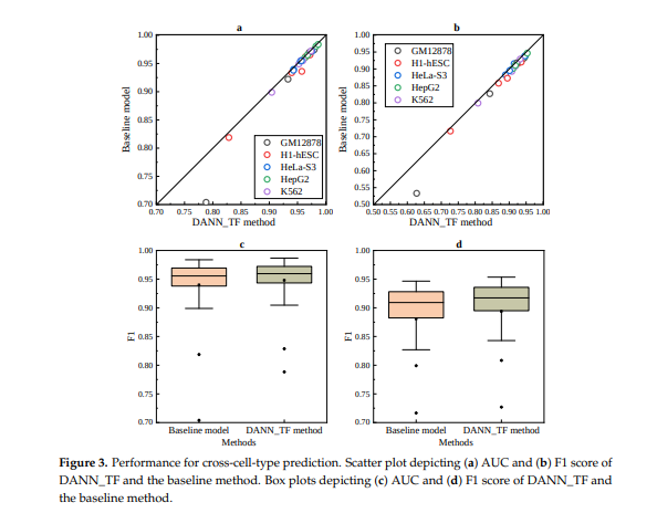
Cross-Cell Type Prediction에 대하여 비교하였을 때에도, 훨씬 성능이 좋은 것을 확인할 수 있다.

2.7. Comparison between Cross-Cell-Type Prediction by DANN_TF and Supervised Prediction by the Baseline Method

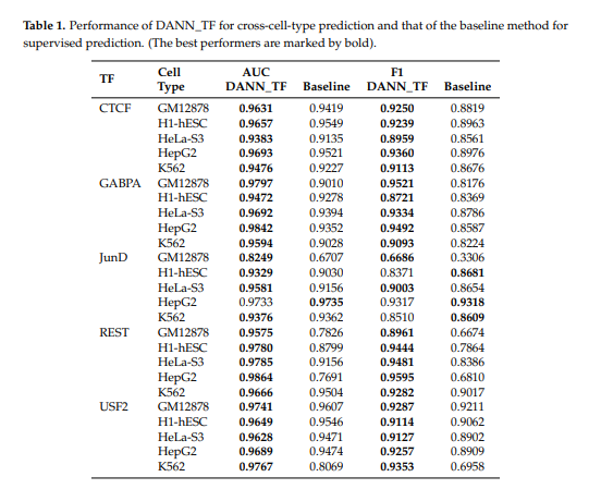
가장 주목할 만한 결과이다. DANN_TF는 Cross-Cell Type으로서 Target Cell에 대한 Label이 없이 Prediction한 결과이고, BaseLine은 Supervised로서 Target Cell에 에대하여 Label을 포함하여 Prediction한 결과이다.

• 23 Cell-type pairs: DANN_TF가 성능이 더 좋다.
• H1-hESC_JunD, K562_JunD: DANN_TF가 AUC는 좋으나, F1은 낮다.
• HepG2_JunD: BaseLine이 성능이 더 좋다.

Label이 없어도 성능이 더 좋다는 것을 확인할 수 있었다.

Real Experiment

1 pair Cell-Type pair에 대하여 Trainng시간이 One-Hot-Encoding: 1.5 + Model Trainning: 4하여 5.5시간 정도가 걸린다. 또한 BaseLine과 비교하기 위하여 실행하게 되면, 1 pair Cell type pair에 대하여 10시간 정도가 걸려 모든 Experiment를 실행하기 위해서는 5(Cell Type) * 5(TF) * 5(Experiment) = 125 따라서 1250시간정도가 걸려서 모든 Experiemnt는 실행하지 못하였고 일부분만 실행하고 확인하였습니다.

Transcription Factor: JunD
Cell Type: GM12878, H1-hESC, HeLa-S3, HepG2, K562

Experiment 1: Comparison of Paper and Experiment
실제 Model이 잘 작동하는지 알아보기 위하여 Paper와 Experiment의 값을 비교하여 알아보자.

• DANN_TF: Cross Cell Type (Label: 0%)
• Baseline: Supervised (Label: 100%)

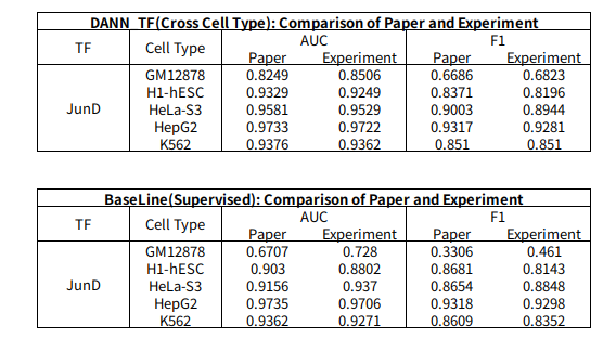
BaseLine의 JunD_GM12878의 결과를 제외하고 차이가 거의 없는 것을 확인할 수 있다. Accuracy가 워낙 낮은 Dataset이므로 차이가 큰 것으로 판단된다.

Experiment2: Comparison of DANN_TF Cross Cell Type and Supervised
DANN_TF Model에서 Cross Cell Type(Label 100%)와 Supervised(Label 0%)의 값을 비교하면 다음과 같다.

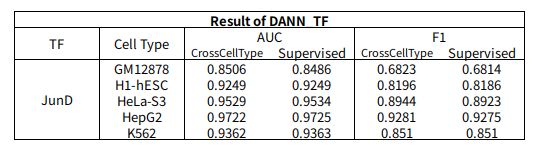
Cross Cell Type과 Supervised의 결과가 거의 차이가 없는 것을 확인할 수 있다.

Experiment3: Comparison of Baseline Cross Cell Type and Supervised
Baseline Model에서 Cross Cell Type(Label 100%)와 Supervised(Label 0%)의 값을 비교하면 다음과 같다.

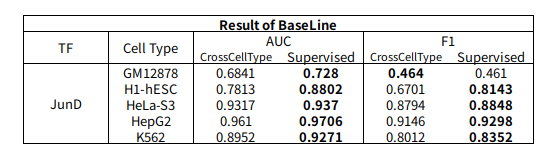
Baseline의 결과를 살펴보게 되면 CrossCellType보다 Supervised가 성능이 훨씬 좋은 것을 살펴볼 수 있다.

Experiment4: Comparison of Baseline Supervised and DANN_TF of Cross Cell Type
Baseline Model의 Supervised(Label 0%)과 DANN_TF의 Cross Cell Type(Label 100%)의 값을 비교하면 다음과 같다.

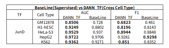
Supervised인 상황에도 불고하고 BaseLine보다 DANN_TF의 성능이 좋은 것을 알 수 있다.

즉, DANN_TF는 Baseline보다 성능이 매우 우수한 것을 살펴볼 수 있고, 또한 Label이 없는 Cross Cell Type에 대하여도 Prediction의 성능이 좋은 것을 알 수 있다.

Appendix

1. Negative Sampling
Dataset을 구축할 당시 TF가 없는 Sequencing도 생성해야 한다. 이러한 방법은 크게 2가지로 나누어질 수 있다.

• Positive Sequencing Data를 Random하게 Shuffle하는 방법이다. => Distribution(A,T,C,G의 개수)가 변하지 않는다는 장점이 있다.
• Label이 달리지 않는 Sequencing을 사용한다.

2가지의 방법을 모두 사용하여 Dataset을 구축하고 Experiment하였으나, 차이가 없다고 말하고 있다.

2. Model Train
논문에서 Cross-Cell-Type을 살펴보면 다음과 같이 실험하였다고 설명하고 있다.

2.6. Results of Cross-Cell-Type Prediction by DANN_TF
To evaluate the performance of cross-cell-type prediction by our proposed DANN_TF, we suppose that all the training data of the target cell type is unlabeled while the validation data as well as the test data are labeled.
Thus, our proposed DANN_TF is trained by combining unlabeled training data of the target cell type and labeled data of source cell types. As the baseline method cannot use unlabeled data, the baseline method is trained by labeled data of source cell types. They are validated and tested by the validation data and the test data of the target cell type, respectively. As our goal is to predict TFBSs of TFs in the target cell type, and DANN_TF is trained by unlabeled training data of the target cell type and labeled data of source cell types, thus DANN_TF is an unsupervised method. For example, when we use DANN_TF to predict TFBSs for CTCF in GM1278, the training data of DANN_TF are the combination of unlabeled training data of CTCF in GM12878 and labeled data of CTCT in other four cell types. As DANN_TF do not use any labeled training data of CTCF in GM12878, predictions of DANN_TF for CTCF in GM12878 are unsupervised predictions.

하지만, 현재 제공한 Code는 다음과 같이 적혀있다.
Supervision mode :
0 : data augmentation method
1 : semi-supervised (10%) method
2 : semi-supervised (20%) method
5 : semi-supervised (50%) method
10 : cross-cell-type method

실제 Model에서는 이러한 supervise라는 Argument로서 Label을 얼만큼 사용할 것인가를 정의하는데, 논문에서 제공하는 Code그대로 실행하게 되면, Data Augmentation과 Cross Cell Type의 Result가 반대로 나오게 될 것이다.

현재 Mail을 보내서 설명이 잘못 작성하였나 물어보았으나, 아직 답변이 없는 상황입니다.

3. BatchSize
Paper에서는 Batch Size를 128이라고 언급하였다. 이에 관하여 BatchSize를 128로 할 시 OOM현상이 발생하여 64로 축소하여 Experiment를 실행하였다.

4. \(\lambda\)
DANN Paper에서는 \(\lambda\)를 다음과 같이 정의하고 있습니다.

$$\lambda= \begin{cases} 1, & \mbox{when }\theta_d \mbox{ update} \\ \frac{2}{1+exp(-10p)-1}, & \mbox{when } \theta_f \mbox{ update, p is 0 to 1 linearly change} \end{cases}$$

하지만, 현재 Code를 살펴보게 되면 다음과 같습니다. l = 1e-3

따라서 다음과 같이 변형하였습니다.

p = float(j) / x_i.shape[0]
l = 2. / (1. + np.exp(-10. * p)) - 1

즉, Iteration을 돌면서 p는 0~1사이의 값을 같게 될 것이고, DANN Paper에서 언급한대로 Sigmoid함수에 적용하여 \(\lambda\)값이 Smooth하게 증가할 것 이다.

5. Change Input PipeLine & Domain Classifier Output
test_4_cross_cell_type.py에서 Domain Classfier가 Source or Target인 2개로서 나누지 않고, 모든 CellType에 구별하도록, 총 5개의 CellType을 구별하도록 다시 구축하였다. 하지만, 결과는 Domain Classifier를 2개로서 구축하는 것 보다 결과가 안 좋았다.

Reference

[1] Domain-Adversarial Training of Neural Networks (https://arxiv.org/pdf/1505.07818.pdf)

[2] A theory of learning from different domains (http://www.alexkulesza.com/pubs/adapt_mlj10.pdf)

[3] Cross-Cell-Type Prediction of TF-Binding Site by Integrating Convolutional Neural Network and Adversarial Network (https://www.ncbi.nlm.nih.gov/pmc/articles/PMC6679139/pdf/ijms-20-03425.pdf)

[4] Jaejun Yoo’s Blog (http://jaejunyoo.blogspot.com/2017/01/domain-adversarial-training-of-neural.html)

[5] GitHub (https://github.com/wjddyd66/others/tree/master/DANN_TF)

코드에 문제가 있거나 궁금한 점이 있으면 wjddyd66@naver.com으로 Mail을 남겨주세요.