Paper02. General DANN:Supervised Adversarial Alignment of Single-Cell RNA-seq Data

Supervised Adversarial Alignment of Single-Cell RNA-seq Data

https://www.biorxiv.org/content/10.1101/2020.01.06.896621v1.full.pdf

Abstract

. The adversarial model tries to simultaneously optimize two objectives.
The first is the accuracy of cell type assignment and the second is the inability to distinguish the batch (domain). We tested the method by using the resulting representation to align several different datasets.
As we show, by overcoming batch effects our method was able to correctly separate cell types, improving on several prior methods suggested for this tas

Single-Cell RNAseq Data에서 scDGN(Single Cell Domain Generalization Network)를 통하여 CellType을 잘 예측하고 Domain에 대한 Batch Effect를 제거하는 것을 목표로 한다.

Dataset

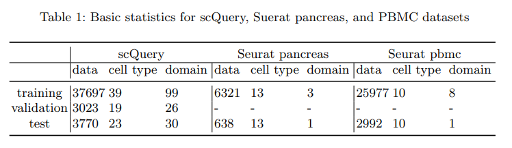
크게 scQuery, Seurat pancreas, PBMC Dataset을 사용하였다. 이 중, Seurat pancreas Dataset의 가장 의미있는 결과를 얻었다고 생각하여 앞으로의 Dataset은 Seurat pancreas로서 설명한다.

실제 Model에 들어가는 Seurat pancreas Dataset을 살펴보게 되면, 다음과 같다.

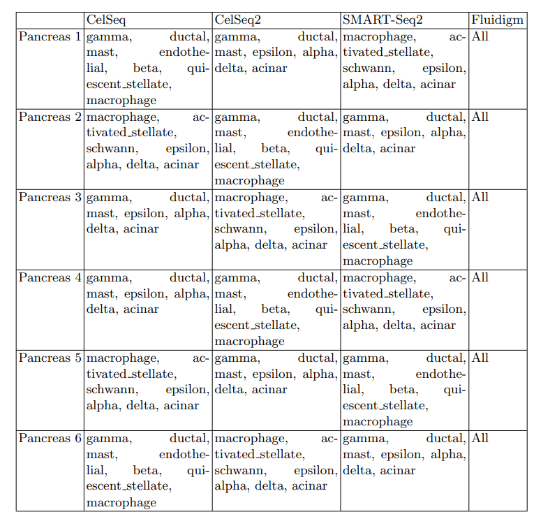
위와 같은 6가지의 Dataset으로서 나누는 과정은 다음과 같다.

1. 3000 most variable genes를 선택
2. The data for 6 of the 13 cell types for each of the training domains
3. Dataset
   • Feature: Num of gene expression: 3000
   • Label: Cell Type => 0~12 ( gamma, ductal, mast, endothelial, beta, quiescentstellate, macrophage, epsilon, alpha, delta, acinar, activated stellate, schwann)
   • Domain: 0~3 => Different sequencing methods (CelSeq, CelSeq2, SMART-Seq2, Fluidigm)

위의 과정으로 인하여 각각의 Dataset의 Domain, Label에 대한 영향과 sample수를 조절해가면서 Experiment를 실행할 수 있다.

Previous Study(DANN Model)

Model

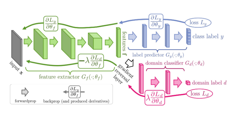
Model을 크게 2개의 Network로서 생각하면 다음과 같다.

• Feature Extractor + Label Predictor: Label Classification Model
• Feature Extractor + Domain Classifier: Domain Classification Model

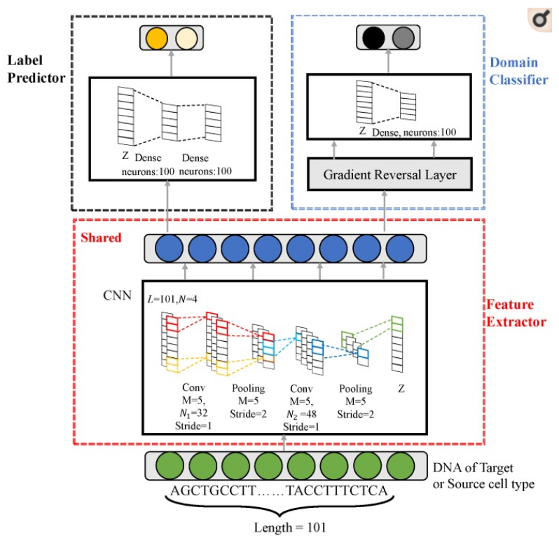
즉, DANN은 Label Classification Model + Domain Classification Model인 Model인 것 이다. 이러한 Model은 크게 다시 3개의 Sub Network를 구별하면 다음과 같다.

• Feature Extractor: Domain에 상관없이 Common한 Feature를 Extraction하는 역할
• Label Predictor: Common한 Feature로서 Label을 Classification하는 역할
• Domain Classifier: Common한 Fuature로서 Domain을 Classification하는 역할

Example)

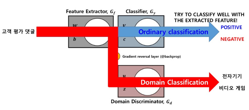
• Probelm: 비디오 게임 고객 평가 댓글이 Positive or Negative인지 Classification하고 싶다. 하지만, 전자기기 고객 평가 댓글 밖에 없는 상황
• Ordinary Classification: 전자기기 고객 평가로서 Model Trainning => 비디오 게임 고객 평가 댓글 Classification
• DANN
  • Label Predictor: 전자기기 고객 평가로서 Trainning
  • Domain Predictor: 전자기기 댓글인지, 비디오 게임 댓글인지 Classification

LossFunction

1. Label Predictor Loss
기존 Classification의 Model 그대로 사용

2. Domain Classifier Loss

$$\hat{d_{\mathcal{H}}}(S,T) = 2 (1-min_{\eta \in \mathcal{H}} [\frac{1}{n}\sum_{i=1}^{n} I[\eta(x_i)=1] + \frac{1}{n^{'}}\sum_{i=n+1}^{N}I[\eta(x_i)=0]])$$

Cross Entropy 로서 구성

3. Total Loss

• \(G_f: \text{Feature Extractor, }G_y: \text{Label Predictor, }G_d: \text{Domain Classifier }\)
• \(\theta_f: \text{Feature Extractor Weight, }\theta_y: \text{Label Predictor Weight, }\theta_d: \text{Domain Classifier Weight }\)
• \(L_y: \text{Label Predictor Loss, }L_d: \text{Domain Classifier Loss }\)
• \(\hat{\theta_f},\hat{\theta_y},\hat{\theta_d}\): Saddle Point

$$E(\theta_f,\theta_y,\theta_d)=\frac{1}{n}\sum_{i=1}^n\mathcal{L}^i_y(\theta_f,\theta_y)-\lambda\left( \frac{1}{n}\sum_{i=1}^n\mathcal{L}^i_d(\theta_f,\theta_d) + \frac{1}{n'}\sum_{i=n+1}^N\mathcal{L}^i_d(\theta_f,\theta_d) \right)$$

$$\begin{align} &(\hat{\theta_f}, \hat{\theta_y}) = \underset{\theta_f,\theta_y}{arg\min} ~E(\theta_f,\theta_y,\hat{\theta_d}), \\ &\hat{\theta_d}= \underset{\theta_d}{arg\max} ~E(\hat{\theta_f},\hat{\theta_y},\theta_d). \end{align}$$

위와같은 Loss를 정의하였다면, Weight Update는 다음과 같이 이루워진다.(u=learning rate)

$$\theta_f \leftarrow \theta_f -u(\frac{\partial L_y^i}{\partial \theta_f} -\lambda \frac{\partial L_d^i}{\partial \theta_f})$$

$$\theta_y \leftarrow \theta_y -u\frac{\partial L_y^i}{\partial \theta_y}$$

$$\theta_d \leftarrow \theta_d -u\lambda \frac{\partial L_d^i}{\partial \theta_d}$$

$$\lambda= \begin{cases} 1, & \mbox{when }\theta_d \mbox{ update} \\ \frac{2}{1+exp(-10p)}-1, & \mbox{when } \theta_f \mbox{ update, p is 0 to 1 linearly change} \end{cases}$$

최종적인 위의 식을 살펴보게 되면, DomainClassifier의 Loss가 Feature Extractor에 갈때는 Loss의 부호가 반대가 되는 것을 확인할 수 있다. 또한 \(\lambda\)값을 0~1로서 Smooth하게 올리는 이유에 관해서는 정확한 설명이 없으나, TFBs를 어느정도 Prediction할 수 있는 상황에서 => Feature를 어느정도 뽑을 수 있는 상황에서 Domain에 상관없는 Domain Independent Feature를 뽑게할 수 있도록 기대할 수 있다.

DANN Model Problem

Paper: DANN_TF Model

• TF: JunD
• CellType: GM12878, H1-hESC, HeLa-S3, HepG2, K562
• Probelm: K562의 Sequencing에 JunD가 Binding or Not Binding
• Source Dataset: GM12878, H1-hESC, HeLa-S3, HepG2
• Target Dataset: K562

My Solution
Target Cell과 Source Cell로서 Domain을 나누는 것은 General한 Model이 아니기 때문에, 모든 Cell Type을 구분하는 Model로서 성능 비교
단순한 softmax cross entropy loss function로서는 General한 Model을 만들 수 없다. => 해당 Paper는 새로운 Loss Function을 사용하여 Model을 구축하여 성능을 향상시켰다.

scDGN(Single Cell Domain Generalization Network)

DANN의 Problem이였던 단순한 softmax cross entropy lossfunction으로서는 General한 Model을 만들 수 없어서 논문에서 말하는 Model은 다음과 같다.

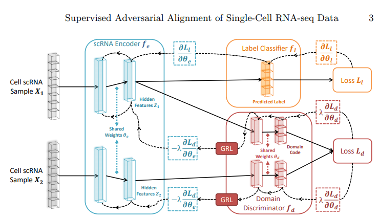
1. 단순하게 Source, Target으로 나누는 것이 아닌 Sampling을 통하여 한 Dataset(\(\text{Cell scRNA Sample} X_1\))에 대해서는 Label Classification과 Domain Classification을 적용한다.
2. 다른 Dataset(\(\text{Cell scRNA Sample} X_1\))에 대해서는 Domain Classfiction만 적용한다.
3. \(\text{Label Classification Model}(X_1)\)을 통하여 Weight Update를 실시한다. (Ordinary Classification Model)
4. \(\text{Domain Classification Model}(X_1), \text{Domain Classification Model}(X_2)\)의 두 값에 대하여 Contrastive loss를 적용한다.

Contrastive Loss

Softmax CrossEntropy Loss Function을 사용하는 경우, 클래스에 따라서 HyperPlane으로서 Classification을 하게 된다. 그 이상으로서 의미있게 학습이 진행되지 않는다는 단점이 있다.
Contrastive Loss는 두 Feature Embedding값 간의 Distance를 계산하는 방식이다. 두 Feature Embedding값이 동일한 Class에 속하는지 여부에 따라 거리값에 대한 손실값 할당을 다르게 하여 Embedding Space의 Distance를 조절한다.

$$L(x_0, x_1, y) = y|f(x_0)-f(x_1)|+(1-y)max(0,m-|f(x_0)-f(x_1)|)$$

• y
  • Same Domain => 1
  • Different Domain => 0
• m: Margin

if y = 1
Term2 = 0 -> \(|f(x_0)-f(x_1)|\): 같은 Domain의 Feature Embedding의 Distance는 가까워 지게 학습을 진행한다.

if y = 0
Term1 = 0 -> \(max(0,m-|f(x_0)-f(x_1)|)\): 다른 Domain의 Feature Embedding의 Distance는 Margin이상이 되도록 학습하게 된다.

위와 같은 Loss를 구축하기 위하여 \(X_0, X_1\)의 Pair를 다음과 같이 정의하였습니다.

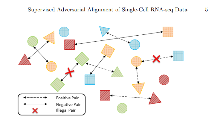
• Shape: Labels(Cell Type)
• Color: Domain(Method of Sequencing)
• Positive Pair: Same Domain but Different Cell Type
• Negative Pair: Different Domain but Same Cell Type

위와 같은 Dataset의 Pair를 Contrastive Loss에 적용하게 되면, 같은 Domain끼리는 Distance가 가까워 지게 되고 다른 Domain끼리는 Distance가 멀어지게 될 것이다.

하지만 Domain Classifier는 Gradient Reverse Layer를 통하여 Gradient가 값이 반대로 Backpropagation이 진행되므로, Feature Embedding Space에서 살펴보면 다음과 같이 Cluster형태로 되어있을 것 이다. => Domain에 대한 정보는 없어지면서 Cell Type에 대한 정보만 남게 되므로 Domain과 상관없이 같은 Cell Type끼리 거리가 가깝게 위치 할 것 이다. 따라서, 처음 목표하였던, Domain Batch Effect는 사라지게 된다.

Contrastive Loss Code

$$L(x_0, x_1, y) = y|f(x_0)-f(x_1)|+(1-y)max(0,m-|f(x_0)-f(x_1)|)$$

class ContrastiveLoss(nn.Module):
    """
    Contrastive loss
    Takes embeddings of two samples and a target label == 1 if samples are from the same class and label == 0 otherwise
    """
    def __init__(self, margin):
        super(ContrastiveLoss, self).__init__()
        self.margin = margin
    def forward(self, output1, output2, target, use_domain, size_average=True):
        distances = (output2  - output1).pow(2).sum(1)+0.001  # squared distances
        losses = 0.5 * (target.float() * distances +
                        (1 +  -1 * target).float() * F.relu(self.margin  - distances.sqrt()).pow(2))
        losses = losses*use_domain
        return losses.mean() if size_average else losses.sum()

• output1: \(\text{DomainClassifier}(X_1)\)
• output2: \(\text{DomainClassifier}(X_2)\)
• target
  • if positive pair: 1
  • if negative pair: 0
• use_domain
  • if illegal pair: 0
  • if not illegal pair: 1
• distance: \((f(x_0)-f(x_1))^2\)

참고 scDGN Model

Model

class scDGN(nn.Module):
    def __init__(self, d_dim=20499, dim1=1136, dim2=100, dim_label=75, dim_domain=64):
        super(scDGN, self).__init__()
        self.dim1 = dim1
        self.dim2 = dim2
        self.d_dim = d_dim
        self.dim_label = dim_label
        self.dim_domain = dim_domain
        self.feature_extractor = nn.Sequential(
           nn.Linear(self.d_dim, self.dim1),
           nn.Tanh(),
           nn.Linear(self.dim1, self.dim2),
           nn.Tanh(),
        )
        self.domain_classifier = nn.Sequential(
            nn.Linear(self.dim2, self.dim_domain),         
            nn.Tanh(),
        )
        self.label_classifier = nn.Sequential(
            nn.Linear(self.dim2, self.dim_label),
        )
        print(self)
    def forward(self, x1, x2=None, mode='train', alpha=1):
        feature = self.feature_extractor(x1)
        reverse_feature = ReverseLayerF.apply(feature, alpha)
        class_output = self.label_classifier(feature)
        if mode == 'train':
            domain_output1 = self.domain_classifier(reverse_feature)
            feature2 = self.feature_extractor(x2)
            reverse_feature2 = ReverseLayerF.apply(feature2, alpha)
            domain_output2 = self.domain_classifier(reverse_feature2)
            return class_output, domain_output1, domain_output2
        elif mode == 'test':
            return class_output
        elif mode == 'eval':
            return feature

• feature_extractor: 간단한 ANN으로서 Feature를 뽑아내게 된다.
• class_output: x1에 대하여 Label에 대하여 Prediction하게 된다.
• domain_output: reverse_feature를 통하여 GRL을 구현하게 되고, x1, x2에 대하여 각각의 Output값을 Return하는 것을 확인할 수 있다.

GRL(Gradient Reberse Layer)

from torch.autograd import Function

class ReverseLayerF(Function):

    @staticmethod
    def forward(ctx, x, alpha):
        ctx.alpha = alpha
        return x.view_as(x)

    @staticmethod
    def backward(ctx, grad_output):
        output = grad_output.neg() * ctx.alpha
        return output, None

Forward는 그대로 값을 전달하지만, Backward에서는 .neg()를 붙여서 부호가 반대로 되는 것을 알 수 있다.

Result

Result of Accuracy

Trainning시에 고려해야 하는 것은 크게 2가지이다. 1)Margin을 어떻게 설정해야 하는가? 2)Domain Classifier -> Feature Extractor의 Backpropation의 양을 어떻게 설정해야 하는가?
아래 결과는 위에서 언급한 2가지의 고려사항을 random하게 Initialization하여 서로 다른 Model에 대한 Accuracy(Prediction of Cell Type)를 비교한 결과이다.(10번 Trainning하고 가장 높은 Accuracy에 대하여 비교)

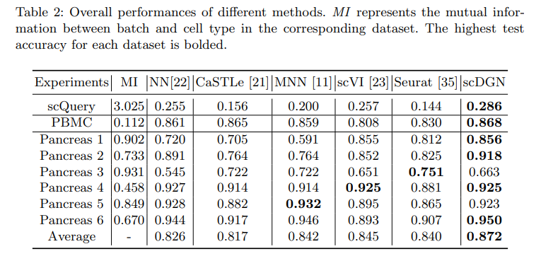
1. Mutual Information
현재 TrainDataset에서 Label, Domain에 대하여 Mutual Information을 직접 구하였다.

$$I(X;Y) = \sum_{y} \sum_{x} p(x,y)log(\frac{p(x,y)}{p(x)p(y)})$$

위의 식을 익숙한 Entorpy로서 표현하면 다음과 같이 나타낼 수 있다.

$$H(X) = \sum_{x}p(x)log(x), H(Y) = \sum_{y}p(y)log(y)$$

$$H(X,Y) = \sum_{x,y}p(x,y)log(p(x,y))$$

$$I(X;Y) = H(X) + H(Y) - H(X,Y)$$

Joint Entropy인 H(X,Y)는 X,Y가 Independent인 경우 H(X)+H(Y)의 값을 가지게 된다. 따라서 Mutual Information으로서 서로다른 두 확률변수의 관계를 통해 압출될 수 있는 정보량을 나타낼 수 있다.

Mutual Information관점에서 NN과 scDGN의 결과를 비교하게 되면, Mutual Information의 값이 높을수록(Label과 Domain의 정보가 서로 압축되어 표현될 수 있는 정보량이 많을수록) Model의 성능이 낮아지는 것을 알 수 있다. 하지만, scDGN은 Mutual Information과 상관 없는 것을 살펴볼 수 있다. 즉, Domain의 Batch Effect를 제거하므로서 Mutual Information이 관계가 없는 것을 알 수 있다. 하지만, Pancreas 3에 관해서는 성능이 낮은 것을 알 수 있다.

2. Numof Dataset
주목해야할 점은 Pancreas3에 대해서는 scDGN의 성능이 안좋은 것을 살펴볼 수 있다.
이에 관하여 실제 Dataset의 개수를 살펴보면 다음과 같다.

• Pancreas 1
  • Train: 2490, Test: 638
• Pancreas 2
  • Train: 2895, Test: 638
• Pancreas 3
  • Train: 1978, Test: 638
• Pancreas 4
  • Train: 4104, Test: 638
• Pancreas 5
  • Train: 2904, Test: 638
• Pancreas 6
  • Train: 3235, Test: 638

Dataset이 적을 경우에는, Model의 성능이 잘 나오지 않는다는 것을 확인할 수 있다.

Visualization of learned representations for NN and scDGN

최종적인 목적은 BatchEffect를 제거하는 것 이므로 위의 Table인 Accuracy의 성능이 아니다. 따라서 다음과 같은 Visualization을 통하여 다시한번 결과를 확인하게 된다.

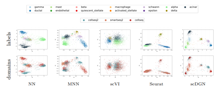
위의 결과는 Feature Extractor에서 나온 Feature를 PCA를 통하여 2차원으로서 줄인뒤 Visualization을 한 것 이다.
결과를 보게 되면, Domain에 대해서는 잘 구별하지 못하지만, CellType에 대해서는 구별을 잘하는 것을 살펴볼 수 있다.

참조 Compute Mutual Information Code

def compute_MI(x, y):
    sum_mi = 0.0
    x_value_list = np.unique(x)
    y_value_list = np.unique(y)
    Px = np.array([ len(x[x==xval])/float(len(x)) for xval in x_value_list ]) #P(x)
    Py = np.array([ len(y[y==yval])/float(len(y)) for yval in y_value_list ]) #P(y)
    for i in range(len(x_value_list)):
        if Px[i] ==0.:
            continue
        sy = y[x == x_value_list[i]]
        if len(sy)== 0:
            continue
        pxy = np.array([len(sy[sy==yval])/float(len(y))  for yval in y_value_list]) #p(x,y)
        t = pxy[Py>0.]/Py[Py>0.] /Px[i] # log(P(x,y)/( P(x)*P(y))
        sum_mi += sum(pxy[t>0]*np.log2( t[t>0]) ) # sum ( P(x,y)* log(P(x,y)/( P(x)*P(y)) )
    return sum_mi, scipy.stats.entropy(Px, base=2), scipy.stats.entropy(Py, base=2)

argument

• x: Trainning Datset of Label
• y: Trainning Dataset of Domain

Reference

[1] Domain-Adversarial Training of Neural Networks (https://arxiv.org/pdf/1505.07818.pdf)

[2] A theory of learning from different domains (http://www.alexkulesza.com/pubs/adapt_mlj10.pdf)

[3] Cross-Cell-Type Prediction of TF-Binding Site by Integrating Convolutional Neural Network and Adversarial Network (https://www.ncbi.nlm.nih.gov/pmc/articles/PMC6679139/pdf/ijms-20-03425.pdf)

[4] Supervised Adversarial Alignment of Single-Cell RNA-seq Data (https://www.biorxiv.org/content/10.1101/2020.01.06.896621v1.full.pdf)

[5] GitHub (https://github.com/wjddyd66/others/tree/master/SupervisedAdversarialAlignmentOfSingle-Cell-RNA-seqData)

코드에 문제가 있거나 궁금한 점이 있으면 wjddyd66@naver.com으로 Mail을 남겨주세요.