
Paper14. TRUSTED MULTI-VIEW CLASSIFICATION
TRUSTED MULTI-VIEW CLASSIFICATION
출처: TRUSTED MULTI-VIEW CLASSIFICATION
코드: hanmenghan Github
Abstract
Multi-view classification (MVC) generally focuses on improving classification accuracy by using information from different views, typically integrating them into a unified comprehensive representation for downstream tasks. However, it is also crucial to dynamically assess the quality of a view for different samples in order to provide reliable uncertainty estimations, which indicate whether predictions can be trusted. To this end, we propose a novel multi-view classification method, termed trusted multi-view classification, which provides a new paradigm for multi-view learning by dynamically integrating different views at an evidence level. The algorithm jointly utilizes multiple views to promote both classification reliability and robustness by integrating evidence from each view. To achieve this, the Dirichlet distribution is used to model the distribution of the class probabilities, parameterized with evidence from different views and integrated with the DempsterShafer theory. The unified learning framework induces accurate uncertainty and accordingly endows the model with both reliability and robustness for out of distribution samples. Extensive experimental results validate the effectiveness of the proposed model in accuracy, reliability and robustness.
Multi-View Classifcation을 사용하는 이유는 여러 Modality를 통하여 해당 Task에 Comprehensive representation으로 나타내어 Classification의 성능을 높이기 위해서 이다. 해당 논문에서 제시하고 있는 의문점은 각각의 sample마다, Modality에 대한 quality가 다르다는 것 이다. 즉, out-of distribution samples를 comprehensive representation에서 발견하는 것이 아닌 각 Modality에서 발견하고 이를 통하여 classificaiton성능 뿐만 아니라 robustness까지 제공하는 Model이라는 것 이다.
Introduction
이전까지의 Multi-View Classification Model을 살펴보게 되면, Comprehensive representation으로 나타내기 위하여 DNN기반의 Model을 많이 사용하게 되었다. 이로 인하여 Model은 점차 Complex해지고 이로 인하여 Interpretable하기 어렵고 또한, Confidence를 구할 수 없었다. 즉, 해당 논문은 이러한 Model에 대하여 다음과 같은 의문을 가지고 있다.
“How confident is the decision?” and “Why is the confidence so high/low for the decision?”
이러한 문제를 해결하기 위한 Model을 제시하고 있으며 다음과 같은 큰 4개의 Contribution을 가지고 있다고 이야기 하고 있다.
(1) We propose a novel multi-view classification model aiming to provide trusted and interpretable (according to the uncertainty of each view) decisions in an effective and efficient way (without any additional computations and neural network changes), which introduces a new paradigm in multi-view classification. 가장 큰 Contribution이라고 생각한다. 제안하는 Model은 단순히 Classification이 성능을 높인 것 뿐만 아니라, Interpretable하고 Trusted하다.
(2) The proposed model is a unified framework for promising sample-adaptive multi-view integration, which integrates multi-view information at an evidence level with the DempsterShafer theory in an optimizable (learnable) way. 단순한 Fusion방법이 아닌 sample-adaptive multi-view integration방법이다.
(3) The uncertainty of each view is accurately estimated, enabling our model to improve classification reliability and robustness.
(4) We conduct extensive experiments which validate the superior accuracy, robustness, and reliability of our model thanks to the promising uncertainty estimation and multi-view integration strategy.
Related Work
Uncertainty-based Learning 기본적으로 우리가 많이 알고 있는 DNN 기반의 Network는 Uncertainity가 아닌, Deterministic function으로서 이루워져 있다. 즉, 각각의 Class에 대한 확률만 나와있고, 그로인하여 그 각 Class에 대한 Confidence는 구할 수 없다.
Uncertainity-based Learning에서 가장 잘 알려진 Network로서는 Bayesian Network가 있으며, 다음과 같은 그림으로서 나타낼 수 있다.
 출처: Uncertainty estimation for Neural Network — Dropout as Bayesian Approximation
즉, weight를 discrete한 값이 아니라, Distribution으로서 나타낼 수 있다면, 각 Class에 대한 확률 뿐만이 아닌, Confidence까지 구할 수 있으므로, 예측하는 과정에서 더 신뢰성을 줌과 동시에 Generalization에 대한 객관적인 지표로서 사용할 수 있다는 것 이다.
비교군으로서 가장 최근에 나온 논문으로서는 Uncertainty Estimation Using a Single Deep Deterministic Neural Network의 예시를 들고 있으며, 설명은 아래 그림과 같다.
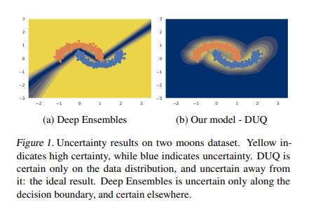
Uncertainity-based Learning으로서 Ensemble로서 Network를 구성할 수 있지만, Dataset을 제외한 부분에 대하여 Confidence Level이 높게 측정되는 결과를 보여주게 된다. 해당 Paper에서는 그러한 문제점을 해결하기 위하여 Distance기반으로서 Model을 구성한다. (아직, 자세히 읽어보지 않았습니다.)
Multi-View Learning 전통적인 방법인, CCA나 MF로서 Multi-Modality를 하나의 Latent Representation으로서 나타낼 수 있다. 최근에는 Siame Network혹은, Triplenet Loss와 같은 Constrative learning을 기반으로 하는Contrastive Multiview Coding로서도 Multi-View Learning에서 좋은 Performance를 보여주고 있다.
Dempster-Shafter Evidence Theory(DST) 해당 논문에서는 Bayesian Network의 Genralization이라 할수 있는 DST를 사용한다. DST의 자세한 내용과 설명은 Dempster-Shafer 이론을 이용한 강우빈도분석 및 불확실성의 정량화의 논문에 나와있으며, 아직 완벽히 이해하지 못하여 따로 설명을 적어두지는 않았습니다.
Trusted Multi-View Classification
Uncertainty and the thory of evidence
먼저 해당 논문의 예시를 알기 위해서는 Dirichlet distribtutions의 예시를 보고 오시면 이해가 쉽습니다.
해당 논문에서는 다음과 같은 Classification Step을 이루고 있습니다.
먼저 한개의 Modality라고 가정하고 Step-by-Step으로 따라가면 다음과 같은 과정을 거치게 됩니다.
- Notation:
- \(K\): Num of Class, \(v\): vth modality, \(u\): Uncertainty
- Evidence \(e^v = [e_1^v, e_2^v, \cdots, e_K^v]\)을 Input으로 받는다.
- Evidence \(e^v\)을 통하여 Dirichlet Distribution인 \(\sum_{i=1}^K(e_i^v+1) = \sum_{k=1}^{K}\alpha^v\)을 구한다.
- 2의 과정을 통하여 Probability로 나타내기 위하여 \(S^v = \sum_{k=1}^K \alpha_i^v\)를 구한다.
- 3의 과정을 통하여 얻은 \(S^v\)를 통하여 \(b_k^v = \frac{e_k^v}{S^v} \rightarrow u^v + \sum_{k=1}^k b_k^v = 1\)을 구한다.
- 각 Class에 대한 확률은 \(\hat{p_k^v} = \frac{\alpha_k^v}{S^v}\)로서 구할 수 있고, Uncertainty는 \(U_v = \frac{K}{S^v}\)로서 구할 수 있다.
먼저 해당 논문에서 예시로 드는 Figure를 보면 이해가 쉽습니다. 아래 Figure는 논문에서 제시하는 예시입니다.
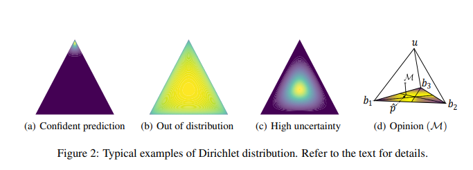
위의 Figure에서 노란색일수록 High Confidence를 말하게 되고, 노란색일 수록 Low Condidence를 의미한다. (a)~(c)의 예시를 살펴보면 다음과 같다. (모든 예시는 Modality가 1개 이고, Num of Class K = 3이라고 가정한 예시입니다.)
(a)Confident Prediction
EX) Evidence \(e = [40, 1, 1]\)로서 한 Class에 대한 Evidence가 큰 예시이다.
\(e = [40, 1, 1] \rightarrow \alpha = [41, 2, 2], S = \sum_{i=1}^{K}\alpha_i = 45\)
\(\rightarrow u = \frac{3}{45} \approx 0.067, p_1 = \frac{41}{45} \approx 0.911, p_2 = \frac{2}{42} \approx 0.045, p_3 = \frac{2}{45} \approx 0.045\)
Class=1일 확률은 0.911로서 매우 높고, 또한 Uncertainty도 0.067로서 매우 낮은 것을 알 수 있다.
(b)Out of distribution
EX) Evidence \(e = [0.0001, 0.0001, 0.0001]\)로서 한 Class에 대한 Evidence가 큰 예시이다.
\(e = [0.0001, 0.0001, 0.0001] \rightarrow \alpha = [1.0001, 1.0001, 1.0001], S = \sum_{i=1}^{K}\alpha_i = 3.0003\)
\(\rightarrow u = \frac{3}{3.0003} \approx 1, p_1 = \frac{1.0001}{3.0003} \approx 0.333, p_2 = \frac{1.0001}{3.0003} \approx 0.333, p_3 = \frac{1.0001}{3.0003} \approx 0.333\)
Class=1, 2, 3일 확률은 0.333이지만, Uncertainty도 1로서 매우 높은 것을 알 수 있다. 즉, Softmax로서 판단하는 경우에는 확률이 0.333이지만 Uncertainty는 1로서 Confidence가 매우 낮은 것을 알 수 있다.
(c)High uncertainty
EX) Evidence \(e = [5, 5, 5]\)로서 한 Class에 대한 Evidence가 큰 예시이다.
\(e = [5, 5, 5] \rightarrow \alpha = [6, 6, 6], S = \sum_{i=1}^{K}\alpha_i = 18\)
\(\rightarrow u = \frac{3}{18} \approx 0.167,p_1 = \frac{6}{18} \approx 0.333, p_2 = \frac{6}{18} \approx 0.333, p_3 = \frac{6}{18} \approx 0.333\)
Class=1, 2, 3일 확률은 0.333이지만, (b)에 비하여 Uncertainty도 0.167로서 (b)보다 낮은 것을 알 수 있다. 즉, Softmax로서 판단하는 경우에는 확률이 0.333으로서 (b)와 같지만, 해당 결과는 (b)보다 더 믿을 수 있는 결과인 것을 확인할 수 있다.
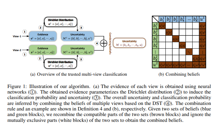
Demster’s rule of combination for multi-view classification
Uncertainty and the thory of evidence는 하나의 Modality에 대한 결과이다. 여러 Modality가 되는 경우에는 다음과 같이 이루워진다.
Example of 2 Modality
해당 Formula는 Figure1에 Step4에 대한 결과이다. 갈색에 대한 값을 구하고, 하얀 값에 대해서는 배제하는 식 이다.
$$\mathcal{M}^1 = \{\{b_k^1\}_{k=1}^K\, \mu^1\} , \mathcal{M}^2 = \{\{b_k^2\}_{k=1}^K\, \mu^2\}$$
$$\mathcal{M} = \mathcal{M}^1 \oplus \mathcal{M}^2 = \{\{b_k\}_{k=1}^K\, \mu\}$$
$$b_k = \frac{1}{1-C}(b_k^1 b_k^2 + b_k^1 \mu^2 + b_k^2 \mu^1), \mu = \frac{1}{C-1}\mu^1 \mu^2$$
$$C = \sum_{i \neq j} b_i^1 b_j^2$$
위의 식을 살펴보면 다음과 같다.
2Modality에 대하여 Joint로서 K class에 대한 확률과 Uncertainty를 구한다
Example of V Modality
Modality가 2개가 아닌 V개로서 Generalization한 Formular이다.
$$\mathcal{M} = \mathcal{M^1} \oplus \mathcal{M^2} \oplus \cdots \mathcal{M^V}$$
$$\mathcal{M} = \{ \{ b_k \}_{k=1}^K, \mu \}$$
$$S = \frac{K}{\mu}, e_k = b_k \times S \text{ and } \alpha_k = e_k + 1$$
Learning to form options
해당 부분에서는 위에서 설명한 Loss Funciton을 Neural Network에 적용하는 방법이다.
먼저 Conventional Neural-Network의 Cross Entropy Loss를 적용하면 다음과 같다.
$$L_{ce} = - \sum_{j=1}^K y_{ij} log(p_{ij})$$
\(p_{ij}\)는 i-th sample에 j class일 확률이다. \(y_{ij}\)는 i-th sample에 j class인 Label이다.
Conventional Neural-Network는 위와 같은 Loss Function으로서 Update된다.
위의 식을 Dirichlet Distribution으로서 나타내면 다음과 같습니다. (Paper에서는 Adjust Cross Entropy라고 칭하고 있습니다.)
$$L_{ace} = \int [\sum_{j=1}^K -y_{ij}log(p_{ij})] \frac{1}{B(\alpha_i)} \prod_{j=1}^K p_{ij}^{\alpha_{ij}-1} d p_i = \sum_{j=1}^K y_{ij}(\psi(S_i) - \psi(\alpha_{ij}))$$
위와 같은 Loss에 대한 문제점을 논문에서는 다음과 같이 지적하고 있다.
The above loss function ensures that the correct label of each sample generates more evidence than other classes, however, it cannot guarantee that less evidence will be generated for incorrect labels. That is to say, in our model, we expect the evidence for incorrect labels to shrink to 0. To this end, the following KL divergence term is introduced:
위의 손실 함수는 각 샘플의 올바른 레이블이 다른 클래스보다 더 많은 증거를 생성하도록 보장하지만 잘못된 레이블에 대해 더 적은 증거가 생성된다는 것을 보장 할 수는 없습니다. 즉, 일반적인 DNN과 달리 Output을 Probability가 아닌 Score로서 Output을 생성하게 된다. 이러한 과정에서 위와 같은 문제가 발생하게 된다. => Probability로서 나타내게 되면, 해당 Class일 확률이 1이 되면, 자동적으로 다른 Class일 확률은 0으로서 바뀌게 되므로 생각하지 않아도 됬다. 하지만, Score로서 나타내게 되면서 이러한 Probability의 특성이 없어지게 되므로 고려해야 한다.
따라서 해당 논문은 다음과 같은 Loss를 추가하였다.
$$KL[D(p_i | \tilde{\alpha_i}) || D(p_i | 1)] = log(\frac{\Gamma(\sum_{k=1}^K \tilde{\alpha}_{ik})}{\Gamma(K) \prod_{k=1}^K \Gamma(\tilde{\alpha_{ik}})}) + \sum_{k=1}^K (\tilde{\alpha_{ik}}-1)[\psi(\tilde{\alpha_{ik}}) - \psi(\sum_{j=1}^K \tilde{\alpha_{ij}})]$$
행당 Loss에서 \(\tilde{\alpha_i} = y_i + (1-y_i) \odot \alpha_i\)로서 Adjust Parameter로서 지정한다.
위의 Loss를 정리한 Loss는 다음과 같다.
$$L(\alpha_i) = L_{ace}(\alpha_i) + \lambda_t KL[D(p_i | (\tilde{\alpha_i}))||D(p_i|1)]$$
최종적인 Loss는 다음과 같다
$$L_{overall} = \sum_{i=1}^N [L(\alpha_i) + \sum_{v=1}^V L(\alpha_i^v)]$$
위의 식을 간단히 생각하면 아래와 같이 생각할 수 있다.
-
\(\tilde{\alpha_i} = y_i + (1-y_i) \odot \alpha_i\)로서 다른 Class일 확률을 0으로서 학습하는 것이 아닌, 어느정도 Penalty를 줌으로서 Confidence를 지정할 수 있다. \(\alpha\)가 크면 클 수록 아마, 다른 Class일 확률이 커져, 작은 Confidence여도 믿을만한 결과를 추론할 수 있다.
-
\(L(\alpha_i)\)를 통하여 전체적인 Classification과 Confidence를 구할 수 있다.
-
\(\sum_{v=1}^V L(\alpha_i^v)\)을 통하여 각각의 Modality에 대한 Cofidence를 구할 수 있다.
Experiments
주요하게 살펴봐야 하는 결과는 2가지 이다.
Performance Comparison on multi-view data with different levels of noisxe
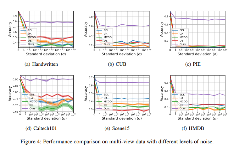
위의 결과를 살펴보게 되면, Noise가 추가되어도, 다른 Model에 비하여 해당 Model의 Performance는 유지되는 것을 살펴볼 수 있다.
Density of uncertainty
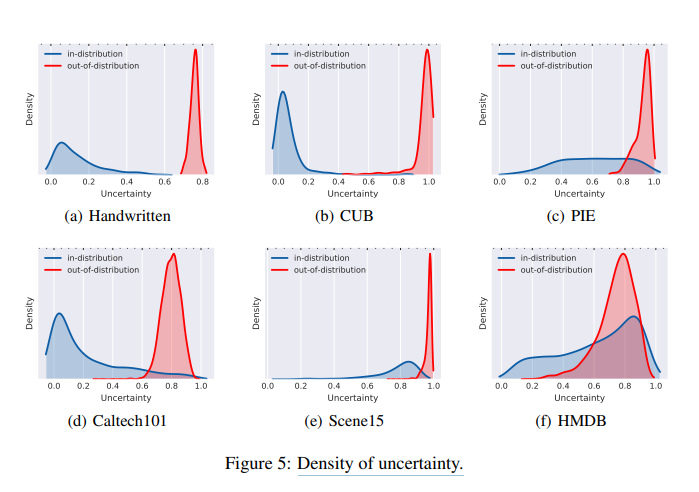
위의 결과를 살펴보게 되면, Uncertainty Threshold에 대한 결과이다. 0.0인 경우에는 Softmax와 동일한 결과이므로, Out-of-distribution 즉, Outlier에 대한 결과를 잘 잡아내지 못하는 것을 확인할 수 있다. Threshold가 높아짐에 따라서 Out-of-Distribution을 잘 찾아내는 것을 확인할 수 있다.
Conclusion
해당 논문에서는 단순히 Classification결과 뿐만 아니라, Confidence를 제공할 수 있다는 것이 제일 중요하다. 또한, 최종적인 Loss를 \(L_{overall} = \sum_{i=1}^N [L(\alpha_i) + \sum_{v=1}^V L(\alpha_i^v)]\)으로서 제공함으로 인하여 단순한 Confidence가 아니라, 각 Modality의 Confidence를 제공할 수 있다는 장점을 가지고 있는 Model이다.
Pytorch Code
출처: Trusted Multi-View Classification Pytorch Code
1
2
3
import torch
import torch.nn as nn
import torch.nn.functional as F
train.py
KL Function
아래 대입한 식은 이해하기 쉽게 Class가 1개일때의 예시이다. 실제 Code는 Num of Class만큼 실행된다.
torch.digamma: \(\psi(x) = \frac{d}{dx}ln(\Gamma(x)) = \frac{\Gamma^{'}(x)}{\Gamma(x)}\)torch.lgamma: \(\text{out}_i = \text{ln}\Gamma(|\text{input}_i|)\)
$$KL[D(p_i | \tilde{\alpha_i}) || D(p_i | 1)] = log(\frac{\Gamma(\sum_{k=1}^K \tilde{\alpha}_{ik})}{\Gamma(K) \prod_{k=1}^K \Gamma(\tilde{\alpha_{ik}})}) + \sum_{k=1}^K (\tilde{\alpha_{ik}}-1)[\psi(\tilde{\alpha_{ik}}) - \psi(\sum_{j=1}^K \tilde{\alpha_{ij}})]$$
alpha: \(\tilde{\alpha_{ij}}\)beta: \(1\)S_alpha: \(\sum_{j=1}^{K} \tilde{\alpha_{ij}}\)-
S_beta: \(\sum_{j=1}^{K} 1\) lnB: \(\text{ln}(\Gamma(\sum_{k=1}^{K} \tilde{\alpha_{ik}}))-\sum_{k=1}^K \text{ln}(\Gamma(\tilde{\alpha_{ik}}))\)-
lnB_uni: \(-\text{ln}(\Gamma(K))\) dg0: \(\psi(\sum_{j=1}^{K} \tilde{\alpha_{ij}})\)dg1: \(\psi(\tilde{\alpha_{ij}})\)torch.sum((alpha - beta) * (dg1 - dg0), dim=1, keepdim=True): \(\sum_{k=1}^K (\tilde{\alpha_{ik}}-1)[\psi(\tilde{\alpha_{ik}}) - \psi(\sum_{j=1}^K \tilde{\alpha_{ij}})]\)
1
2
3
4
5
6
7
8
9
10
11
12
13
14
# loss function
def KL(alpha, c):
    beta = torch.ones((1, c)).cuda()
    S_alpha = torch.sum(alpha, dim=1, keepdim=True)
    S_beta = torch.sum(beta, dim=1, keepdim=True)

    lnB = torch.lgamma(S_alpha) - torch.sum(torch.lgamma(alpha), dim=1, keepdim=True)
    lnB_uni = torch.sum(torch.lgamma(beta), dim=1, keepdim=True) - torch.lgamma(S_beta)

    dg0 = torch.digamma(S_alpha)
    dg1 = torch.digamma(alpha)

    kl = torch.sum((alpha - beta) * (dg1 - dg0), dim=1, keepdim=True) + lnB + lnB_uni
    return kl
ce_loss Function
$$L(\alpha_i) = L_{ace}(\alpha_i) + \lambda_t KL[D(p_i | (\tilde{\alpha_i}))||D(p_i|1)]$$
A: \(\sum_{j=1}^K y_{ij}(\psi(S_i) - \psi(\alpha_{ij}))\)B: \(\lambda_t KL[D(p_i | \tilde{\alpha_i}) || D(p_i | 1)]\)
점차적으로 KL Loss를 증가시키는 방법으로 학습함으로 인하여 KL divergence Loss에 너무많은 Attention이 가해지는 것을 방지하였다.
1
2
3
4
5
6
7
8
9
10
11
12
def ce_loss(p, alpha, c, global_step, annealing_step):
    S = torch.sum(alpha, dim=1, keepdim=True)
    E = alpha - 1
    label = F.one_hot(p, num_classes=c)
    A = torch.sum(label * (torch.digamma(S) - torch.digamma(alpha)), dim=1, keepdim=True)

    annealing_coef = min(1, global_step / annealing_step)

    alp = E * (1 - label) + 1
    B = annealing_coef * KL(alp, c)

    return (A + B)
model.py
Classifier
간단하게 Modality의 개수만큼 Input -> Output(Num of Class)로서 1개의 Dimension을 가지는 Classifier의 집합이다.
1
2
3
4
5
6
7
8
9
10
11
12
13
14
15
class Classifier(nn.Module):
    def __init__(self, classifier_dims, classes):
        super(Classifier, self).__init__()
        self.num_layers = len(classifier_dims)
        self.fc = nn.ModuleList()
        for i in range(self.num_layers-1):
            self.fc.append(nn.Linear(classifier_dims[i], classifier_dims[i+1]))
        self.fc.append(nn.Linear(classifier_dims[self.num_layers-1], classes))
        self.fc.append(nn.Softplus())

    def forward(self, x):
        h = self.fc[0](x)
        for i in range(1, len(self.fc)):
            h = self.fc[i](h)
        return h
TMC
DS_Combine_two Function
$$\mathcal{M}^1 = \{\{b_k^1\}_{k=1}^K\, \mu^1\} , \mathcal{M}^2 = \{\{b_k^2\}_{k=1}^K\, \mu^2\}$$
$$\mathcal{M} = \mathcal{M}^1 \oplus \mathcal{M}^2 = \{\{b_k\}_{k=1}^K\, \mu\}$$
$$b_k = \frac{1}{1-C}(b_k^1 b_k^2 + b_k^1 \mu^2 + b_k^2 \mu^1), \mu = \frac{1}{C-1}\mu^1 \mu^2$$
$$C = \sum_{i \neq j} b_i^1 b_j^2$$
DS_Combine Function
$$\mathcal{M} = \mathcal{M^1} \oplus \mathcal{M^2} \oplus \cdots \mathcal{M^V}$$
$$\mathcal{M} = \{ \{ b_k \}_{k=1}^K, \mu \}$$
$$S = \frac{K}{\mu}, e_k = b_k \times S \text{ and } \alpha_k = e_k + 1$$
1
2
3
4
5
6
7
8
9
10
11
12
13
14
15
16
17
18
19
20
21
22
23
24
25
26
27
28
29
30
31
32
33
34
35
36
37
38
39
40
41
42
43
44
45
46
47
48
49
50
51
52
53
54
55
56
57
58
59
60
61
62
63
64
65
66
67
68
69
70
71
72
73
74
75
76
77
78
79
80
81
82
83
84
85
86
87
88
89
90
91
92
93
class TMC(nn.Module):

    def __init__(self, classes, views, classifier_dims, lambda_epochs=1):
        """
        :param classes: Number of classification categories
        :param views: Number of views
        :param classifier_dims: Dimension of the classifier
        :param annealing_epoch: KL divergence annealing epoch during training
        """
        super(TMC, self).__init__()
        self.views = views
        self.classes = classes
        self.lambda_epochs = lambda_epochs
        self.Classifiers = nn.ModuleList([Classifier(classifier_dims[i], self.classes) for i in range(self.views)])

    def DS_Combin(self, alpha):
        """
        :param alpha: All Dirichlet distribution parameters.
        :return: Combined Dirichlet distribution parameters.
        """
        def DS_Combin_two(alpha1, alpha2):
            """
            :param alpha1: Dirichlet distribution parameters of view 1
            :param alpha2: Dirichlet distribution parameters of view 2
            :return: Combined Dirichlet distribution parameters
            """
            alpha = dict()
            alpha[0], alpha[1] = alpha1, alpha2
            b, S, E, u = dict(), dict(), dict(), dict()
            for v in range(2):
                S[v] = torch.sum(alpha[v], dim=1, keepdim=True)
                E[v] = alpha[v]-1
                b[v] = E[v]/(S[v].expand(E[v].shape))
                u[v] = self.classes/S[v]

            # b^0 @ b^(0+1)
            bb = torch.bmm(b[0].view(-1, self.classes, 1), b[1].view(-1, 1, self.classes))
            # b^0 * u^1
            uv1_expand = u[1].expand(b[0].shape)
            bu = torch.mul(b[0], uv1_expand)
            # b^1 * u^0
            uv_expand = u[0].expand(b[0].shape)
            ub = torch.mul(b[1], uv_expand)
            # calculate C
            bb_sum = torch.sum(bb, dim=(1, 2), out=None)
            bb_diag = torch.diagonal(bb, dim1=-2, dim2=-1).sum(-1)
            C = bb_sum - bb_diag

            # calculate b^a
            b_a = (torch.mul(b[0], b[1]) + bu + ub)/((1-C).view(-1, 1).expand(b[0].shape))
            # calculate u^a
            u_a = torch.mul(u[0], u[1])/((1-C).view(-1, 1).expand(u[0].shape))

            # calculate new S
            S_a = self.classes / u_a
            # calculate new e_k
            e_a = torch.mul(b_a, S_a.expand(b_a.shape))
            alpha_a = e_a + 1
            return alpha_a

        for v in range(len(alpha)-1):
            if v==0:
                alpha_a = DS_Combin_two(alpha[0], alpha[1])
            else:
                alpha_a = DS_Combin_two(alpha_a, alpha[v+1])
        return alpha_a

    def forward(self, X, y, global_step):
        # step one
        evidence = self.infer(X)
        loss = 0
        alpha = dict()
        for v_num in range(len(X)):
            # step two
            alpha[v_num] = evidence[v_num] + 1
            # step three
            loss += ce_loss(y, alpha[v_num], self.classes, global_step, self.lambda_epochs)
        # step four
        alpha_a = self.DS_Combin(alpha)
        evidence_a = alpha_a - 1
        loss += ce_loss(y, alpha_a, self.classes, global_step, self.lambda_epochs)
        loss = torch.mean(loss)
        return evidence, evidence_a, loss

    def infer(self, input):
        """
        :param input: Multi-view data
        :return: evidence of every view
        """
        evidence = dict()
        for v_num in range(self.views):
            evidence[v_num] = self.Classifiers[v_num](input[v_num])
        return evidence
참조: TRUSTED MULTI-VIEW CLASSIFICATION
참조: hanmenghan Github
코드에 문제가 있거나 궁금한 점이 있으면 wjddyd66@naver.com으로 Mail을 남겨주세요.
Leave a comment