Paper20. Multimodal data visualization, denoising and clustering with integrated diffusion

Multimodal data visualization, denoising and clustering with integrated diffusion

출처: Multimodal data visualization, denoising and clustering with integrated diffusion

Abstract

We propose a method called integrated diffusion for combining multimodal datasets, or data gathered via several different measurements on the same system, to create a joint data diffusion operator. As real world data suffers from both local and global noise, we introduce mechanisms to optimally calculate a diffusion operator that reflects the combined information from both modalities. We show the utility of this joint operator in data denoising, visualization and clustering, performing better than other methods to integrate and analyze multimodal data. We apply our method to multi-omic data generated from blood cells, measuring both gene expression and chromatin accessibility. Our approach better visualizes the geometry of the joint data, captures known crossmodality associations and identifies known cellular populations. More generally, integrated diffusion is broadly applicable to multimodal datasets generated in many medical and biological systems.

Multi-Modality를 Visualization하는데 있어서, 어려운점은 크게 2가지 이다.

1. Multi-Modality를 어떻게 통합하여 Visualization할 것 인가?
2. 실제 Bio Data에서는 많은 Noise(Global or Local)을 어떻게 처리할 것 인가?

해당 논문은 이러한 2가지 문제점을 Main Problem으로 선정하고 Integrated Diffusion으로서 해결하였다. 이러한 방법이 효과적인지 보여주기 위하여, Experiment로서 1) Visualization, 2) Denoising, 3) Clustering를 수행하고 결과를 보여준다.

Introduction

Multi-Modality의 Down Stream(Classification, Denoising)등을 사용하기 위하여 Data를 어떻게 Integration을 하는지가 주요하다.

하지만 이러한 Data Integration이 Bio Domain에서는 3가지 어려운점을 가지게 된다.

1. Differently Scale
2. Different amount of Noise
3. Different amount of Sparsity

즉, 실제 Dataset에서는 Noise가 존재하게 되고, 또한 Data Integration에서 Modality Specific Information을 다루기 어렵다는 것이다. 즉, 전통적인 방법인 CCA나 AutoEncoder의 경우에는 Early Fusion으로서 Relationship을 Latent Representation을 나타내는데 효과적이나 Modality Specific Information을 포함하고 있지는 않다.

해당 논문에서는 이러한 문제를 해결하면서 Integrated Difussion을 통하여 Multi-Modality의 Integration을 목표로 하고 있다.

Preliminaries

Manifold Learning

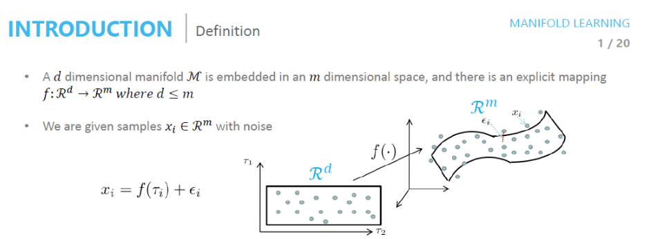
사진 참조: deepinsight 블로그

• \(Z = \{ z_i\}_{i=1}^{N} \subset \mathbb{M}^{d}\): Latent Represenation
• \(X = \{ x_1, \ldots, x_N\} \subset \mathbb{R}^n\)
• \(f(\cdot)\): Embedding Function

Mainfold Learning이라는 것은 \(z_i = f(x_i)\)를 만족하는 \(f(\cdot)\)을 찾아내는 방법이다.
EX) \(f(\cdot) = \text{Linear Function}\): CCA, \(f(\cdot) = \text{Non Linear Function}\): AutoEncoder

Difussion geometry

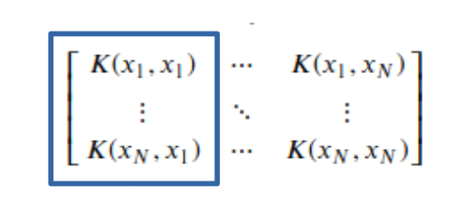
$$\text{K}(x_i, x_j) = \text{exp}(-\frac{\|x_i - x_j\|^2}{\epsilon}), i,j=1, \ldots, N$$

$$\text{P} = \text{D}^{-1} \text{K}$$

• \(\text{P}\): Single Step transition probabilities ofr a time-homogeneous diffusion process, Markovian random walk
• \(\text{D}(x_i, x_j) = \sum_{j} \text{K}(x_i, x_j)\)

위의 식을 이해하기 위해서는 Markov Transition Matrix를 대입해서 이해해야 한다.
\(\text{K}(x_i, x_j) = \text{exp}(-\frac{\|x_i - x_j\|^2}{\epsilon})\)를 Markov Transition Matrix로서 생각하면, \(x_j \rightarrow x_i\)가 될 확률이다. 또한 Matrix를 생각하면 다음과 같은 의미가 있다.

\(p(x_1 | x_1) + p(x_2 | x_1) \cdots p(x_N | x_1) = \sum_{i=1}^N p(x_i | x_1) = 1\): 현재 상태 \(x_1\)에서 다음 상태 x_N이 될 확률의 합

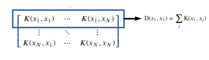
\(p(x_1 | x_1) + p(x_1 | x_2) \cdots p(x_1 | x_N) = \sum_{i=1}^N p(x_1 | x_i)\): 이전 상태와 상관없이 현재 상태 \(x_1\)이 될 확률의 합 -> \(\text{D}^{-1}\)은 Diagonal Matrix로서 Laplacian Regularization을 의미하게 된다.

\(P^t, t > 0\)은 simulate multi-step random walks over the data로서 multiple-step뒤에 \(x_j \rightarrow x_i\)로 될 확률 + Laplacian Regularization(L1 Regularization)을 나타낸다. 즉, 확률이 높으면 높을수록 Mainfold Space상에서 가까운 위치에 존재한다고 말할 수 있다. 또한 t가 크면 클수록 가까운 거리의 Point로서만 이동할 수 있도록 Regularization을 가할 수 있다.

만약, L1 Regularization이 없다면, 해당 Data Point주변을 계속해서 돌게 된다.

Alternating diffusion

$$\text{P}(x_i, x_j) = \text{P}_i * \text{P}_j$$

위의 식은 \(x_i\)Data에 대한 1 moality Markovian random walk(\(\text{P}_i\))와 \(x_j\)Data에 대한 2 moality Markovian random walk(\(\text{P}_j\))의 Product로서 Across Modality에서의 Markovian random walk(Joint difussion map embedding)의 의미하게 된다. 하지만, Modality Specific Information을 잃게 된다.

Method

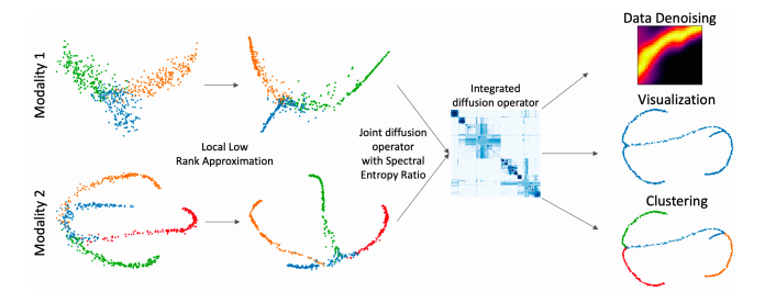
해당 논문에서 제시하는 Method는 위와 같은 과정으로 이루워진다.

1. Local Low rank approximation -> 해당 과정에서는 Dimension이 서로 다른 Modality를 Joint하기 위하여 같은 Dimension의 Low Rank로서 나타내는 것 뿐만아니라 Local Noise를 제거한다.
2. Joint diffusion operator with Spectral Entropy Ratio, Integrated diffusion operator -> 각각의 Modality의 특징을 알아내기 위하여 각 Modality의 Diffusion을 구한뒤 Multi-Modality를 사용하기 위하여 Joint한다.
3. Result(DownStream - Data Denoising, Visualization, Clustering): 해당 논문의 Result를 통하여 Data Denoising, Visualization, Clustering이 가능하다.

Problem Formulation

• \(X \subseteq \mathbb{R}^{D_x}\): Modality 1 Data, Feature Dimension = \(D_x\)
• \(Y \subseteq \mathbb{R}^{D_y}\): Modality 2 Data, Feature Dimension = \(D_y\)
• \(d << \text{min}(D_x, D_y)\): Manifold Dimension = \(d\)

서로 다른 Modality(\(X, Y\))를 Row-Rank이면서 Joint로서 나타낼 수 있는 Latent Representation(d)로 나타내는 것을 목표로 한다.

Neighborhood low rank approximation for local noise correction

1. \(X = X_1, \ldots, X_N\): Data X를 N개의 Group으로서 Clustering을 실시한다.
2. 각 Group에 대하여 \(X_i - \bar{X_i} = U S V^T\)로서 Centering + SVD를 실시한다.
3. \(\tilde{X}_i = U^{'} S^{'} (V^{'})^T + \bar{X_i}\)로서 k+1개의 singular value로서 나타낸다.

해당 과정으로 인하여, Modality에 대한 Noise에 대하여 Locally Denoising이 가능하다. 이러한 결과는 Highly Locally -> 전체적인 Data의 Distribution을 해치지 않으므로 Raw Data -> Manifold 로서의 Mapping또한 크게 해치지 않는다.

Modality specific diffusion time scale calculation via spectral entropy
위에서 언급할 때, \(P^t\)에서 t가 크면 클수록 가까운 거리의 Point로서만 이동할 수 있도록 Regularization을 가할 수 있다. 라고 설명하였다. Spectrum상에서 살펴보면 다음과 같다.

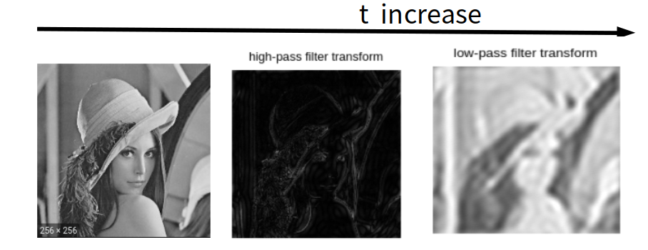
t가 증가함에 따라서, 점진적으로 High-Pass-Filter(해당 Point와 다른 Point까지 Random Walk로서 갈 수 있음)에서 Low-Pass-Filter(해당 Point의 근처 Point까지만 Random Walk로서 갈 수 있음)로서 변한다는 것을 알 수 있다. 해당 논문에서는 적절한 t를 선택하기 위하여 Spectral Entropy를 사용하였다.

Spectral Entropy

$$H(t) = - \sum_{i=1}^N \eta(t)_i \text{log}[\eta(t)]_i$$

• \(\lambda_1, \lambda_2, \cdots, \lambda_k\): Eigenvalues of Each Modality Difussion geometry
• \(\eta(t)\): Sum of Eigenvalues

위의 식에서 K로서 EigenValue를 정한 까닭은 위에서 Neighborhood low rank approximation for local noise correction과정에서도 K개의 Eigenvalue로서 충분히 원본 데이터를 나타낼 수 있다고 가정하였기 때문이다.

즉, 위의 식은 점진적으로 감소되기 때문에 Elbow를 찾고 그것을 Cut-off로서 구성한다.
(t가 증가되면 될수록, Loss는 계속해서 감소되겠지만, Modality에서 중요한 Information을 잃을수 있다.)

또한 해당 논문에서 PCA와의 차이점으로 다음과 같이 설명하고 있다.

In this manner, the higher frequency components of the data graph, corresponding to noise dimensions will be eliminated in a frequency-specific manner globally on the graph, as opposed to locally in a vertex-specific manner using local PCA.

정확히 이해되지 않으나, PCA는 Locally하게 Dimension Reduction을 하는 방법이라고 나와있다. 즉, 분산을 기준으로 큰 것을 찾다 보니, 다음과 같이 이야기 하는 것 같다. 개인적인 생각으로는 PCA또한, 분산을 기준으로 Cut-Off를 잡다보니 High-Pass Filter에서 Low-Pass Filter로서 Filtering하는 Datapoint를 늘리는 것은 동일하다고 생각한다. (아직 자세하게 모르겠습니다.)

Fusion of operators
위에서 정의한 각각의 Modality에 대한 Spectral Entropy를 활용하여 최종적인 식을 적으면 다음과 같다.

$$\text{J} = \text{P}_1^{t_1} * \text{P}_2^{t_2}$$

주요한 점은 \(\text{J} = \text{P}_1^{t} * \text{P}_2^{t}\)로서 사용하면 Modality Specific Information을 잃어버릴 수 있으나 위의 식은 각각의 Modality의 Information의 양을 \(t_1, t_2\)로 나타내었기 때문에 이러한 문제점을 해결하였다.

또한, \(t_1:t_2 = 2:8\)이라면 각 Modality의 Information을 1:4로서 나타낼 수 있다. 즉, t가 증가하면 할수록 LPF로서 그 Modality의 Information을 많이 가지고 있기 때문이다.

Experimental Results

Experiment Setting

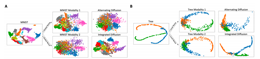
• Dataset1: MNIST + Gaussian Noise(\(p^{'}_i = p_i + N(v)\))
  • Modality1: MNIST + Fix Gaussian Noise (Global Noise)
  • Modality2: MNIST + Increasing Gaussian Noise (Global Noise)
• Dataset2: Tree + Local Noise(Tree Dataset은 Simulation으로서 만든 Data)
  • Modality1: Tree + Fix Gaussian Noise (Global Noise)
  • Modality2: Tree + Increasing Gaussian Noise (Global Noise)
• Dataset3: Single cell biological data measuring RNA-sequencing, or gene expression, and ATAC-sequencing, or chromatin accessibility. (Real-World BioData)

Visualization
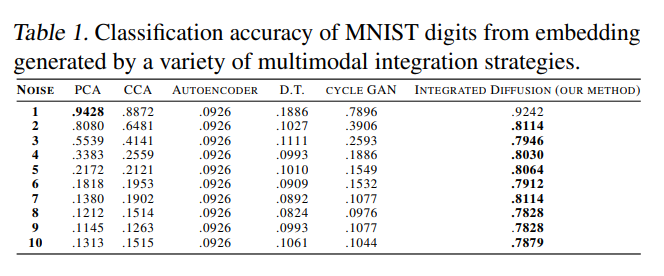
Visualization을 평가하는 방법은 없다. (주관적인 평가만 가능하기 때문에) 따라서 해당 논문에서는 Visualization이 좋은 것은 잘 분류되도록 Embedding된 Latent Representation으로서 만드는 Model이라고 가정하였다. (Classification or Performance가 높은 Model)

1. Global Noise를 추가하였을 경우는 K-NN으로서 Classification 성능을 측정하여 직접적으로 비교 하였다. 기본적으로 잘 알려진 PCA뿐만 아니라 다른 전통적인 Model보다 성능이 좋았다.

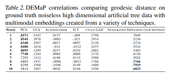
2. Local Noise를 추가하였을 경우의 평가 Metric은 DeMAP(Denoised Embedding Manifold Preservation)을 사용하였다.

Denoising
Denoising 효과를 알아보기 위하여 실제 Noise Data를 얼만큼 잘 Original Data로서 Reconstruction하는지 확인하였다.

1. K-NN Model을 Noise없는 Data로서 학습
2. Noise를 추가한 Data를 평가하고자 하는 Denosing Model의 Input으로 활용
3. Denoising Model Output을 K-NN Model의 Input으로서 Classification 수행

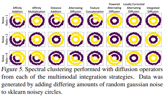
Clustering
Clustering으로서는 기본적으로 많이 사용하는 Moon Dataset으로서 평가하였다.

Biological Applications

• Dataset: Multimodal single cell data of 11909 blood cells
• Modality: Gene Expression, Chromatin Accessibility

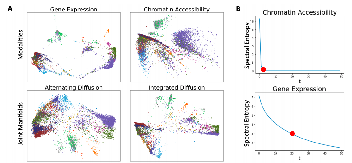
위의 결과(Color=Cell Type)에 대해서는 해당 논문에서 아래와 같이 설명하고 있다.

Chromatin accessibility data, when compared to gene expression data, is incredibly sparse and generally considered to be far less informative.

1. Chromatin Accessibility는 Gene Expression에 비하여 더 Sparse하고 Less infomative하다고 알려져있다. 따라서, 해당 논문의 Method에 설명한 것과 같이 Spectral Entropy에서 t를 비교할때 훨씬 적은 것을 알 수 있다.

2. 기존의 방법 PHATE(Alternating Diffusion)보다 훨씬 Sharp하게 Embedding이 가능하다.

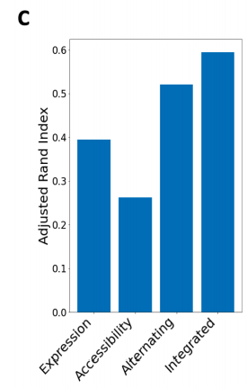
위의 결과는 해당 논문의 Method로 Embedding된 Data를 Clustering Performance Metric을 ARI(Adjusted Rand Index)로서 측정한 것 이다. Multi-Modality로서 Cell Type을 Clustering하는 것이 효과가 크고, 기존의 방법보다 더 성능이 좋은 것을 알 수 있다.

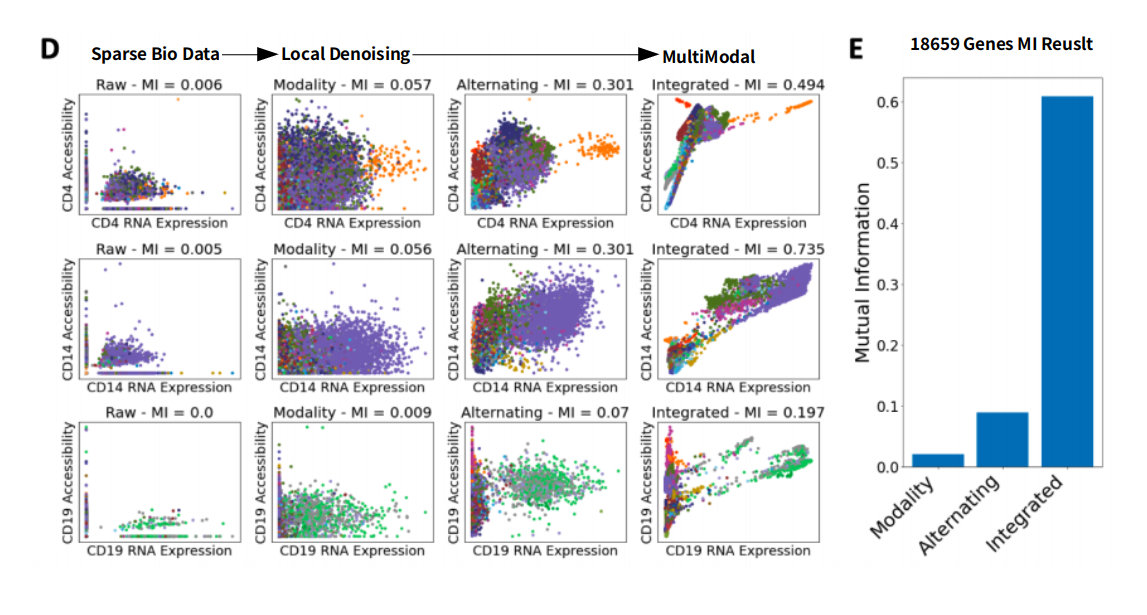
또한 논문은 다음과 같이 설명하고 있다.

Theoretically, if a gene is expressed, then the chromatin encoding that gene must be accessible.

하지만, BioData는 너무 Sparse하므로 위와 같은 결과를 보여주고 있지 않다. 하지만 해당 Method를 사용하면 해결 가능하다.

참조 Adjusted Rand Index

• Rand Index: Taegu Blog
• Adjusted Rand Index: Taegu Blog
• Adjusted Rand Index: p829911 Blog

Conclusion

해당 논문에서는 Graph이론에 접목하여 Multi-Modality의 Visualization을 수행하였다. 해당 논문은 다음과 같은 장점이 있다.

1. 각 Modality의 Information(Important)정도를 나타낼 수 있다.
2. 각 Specific Modality의 Noise를 제거할 수 있음 뿐만 아니라, Specific Modality를 고려하여 Low-Rank로서 나타낼 수 있다.
3. High-Dimension -> Low Dimension으로 나타냄으로 인하여 Classification, DownStream, Visualization등 다양한 DownStream을 사용할 수 있다.

하지만 단점으로서는, 개인적인 Model의 Visualization하기에는 Denoising을 포함하고 있으므로 Model의 Robust정도를 Visualization으로 살펴볼 수 없으며, AutoEncoder와 같이 Modality를 합친 Latent Representation을 Visualization을 하는 방법은 아니다.(Only MultiModality)

---

참조: Multimodal data visualization, denoising and clustering with integrated diffusion
참조: Taegu Blog1
참조: Taegu Blog2
참조: p829911 Blog
참조: deepinsight 블로그

코드에 문제가 있거나 궁금한 점이 있으면 wjddyd66@naver.com으로 Mail을 남겨주세요.