Paper21. DIABLO: an integrative approach for identifying key molecular drivers from multi-omics assays

DIABLO: an integrative approach for identifying key molecular drivers from multi-omics assays

출처: DIABLO: an integrative approach for identifying key molecular drivers from multi-omics assays
코드: singha53 GitHub

Abstract

Motivation: In the continuously expanding omics era, novel computational and statistical strategies are needed for data integration and identification of biomarkers and molecular signatures. We present Data Integration Analysis for Biomarker discovery using Latent cOmponents (DIABLO), a multi-omics integrative method that seeks for common information across different data types through the selection of a subset of molecular features, while discriminating between multiple phenotypic groups.
Results: Using simulations and benchmark multi-omics studies, we show that DIABLO identifies features with superior biological relevance compared with existing unsupervised integrative methods, while achieving predictive performance comparable to state-of-the-art supervised approaches. DIABLO is versatile, allowing for modular-based analyses and cross-over study designs. In two case studies, DIABLO identified both known and novel multi-omics biomarkers consisting of mRNAs, miRNAs, CpGs, proteins and metabolites.
Availability and implementation: DIABLO is implemented in the mixOmics R Bioconductor package with functions for parameters’ choice and visualization to assist in the interpretation of the integrative analyses, along with tutorials on http://mixomics.org and in our Bioconductor vignette. Contact: kimanh.lecao@unimelb.edu.au

DIABLO(Data Integration Analysis for Biomarker discovery using Latent cOmponents)방법은 여러 Multi-Omics Data를 Integration및 Classification에 사용되는 Model이다. 이러한 제안하는 DIABLO Model은 1) Unsupervised Integration방법과비교하여 더 우수한 Multi-Omics간의 관계를 파악할 수 있다. 2) Classification의 성능이 State-Of-The-Art보다 뛰어나다는 것을 알 수 있다.

Introduction

다른 Multi-Modality Model과 유사한 Introduction을 가추고 있다.

먼저, Single-Omics를 사용하는 것보다 Multi-Omics를 사용하는 것이 Improved biological insights를 제공할 수 있다. 왜냐하면 Single-Omics는 Omics layers의 Interaction을 고려할 수 없기 때문이다.

해당 논문에서는 많은 상황에서의 결과를 확인하기 위하여 아래와 같은 직접 Simulation Data와 실제 Real World Dataset을 구별하여 실험을 수행하였다.

해당 Paper는 2가지 주요 Task에 대하여 Experiment를 실시하였다. 1) Multi-Omics Data에서 Unsupervised Integration, 2) Classification이다.
해당 논문은 Multi-Omics Integration의 비교군으로서 JIVE(Joint and Individual Variation Explained), sGCCA(Sparse Generalized Canonical Correlation Analysis), MOFA(Multi-Omics Factor Analysis)와 비교하였다.
또한 Classification + Multi-Omics Integration의 능력을 살펴보기 위하여 Unsupervised Model인 Ensemble, Concatenation-Based Model과 비교하였다.

해당 논문에서 제시하는 DIABLO는 위의 2가지 Task에서 기존의 Model보다 성능이 좋은 것을 확인할 수 있고 또한, Visualization또한 DownStream으로서 매우 잘 수행된다.

Materials and methods

General multivariate integrative framework

$$\max_{a_b^{(1)}, \ldots, a_b^{(Q)}} \sum_{i,j=1, i\neq j}^Q c_{i,j} \text{cov}(X_b^{(i)} a_b^{(i)}, X_b^{(j)} a_b^{(j)})$$

$$\text{s.t. }\|a_b^{(q)}\|_2 = 1 \text{ and } \|a_b^{(q)}\|_1 \le \lambda^{(q)} \text{ for all} 1 \le q \le Q$$

• \(N\): Number of Sample
• \(Q\): Number of Modality
• \(X_b^{(q)}\): Residual Matrix of \(X^{(q)}\)
• \(c_{i,j}\): Matrix that specifies whether datasets should be connected.
• \(\lambda^{(q)}\): Non negative parameter that controls the amount of shrinkage
• \(a_b^{(q)}\): Coefficient

위의 식을 살펴보게 되면, 기본적인 PLS와 식이 똑같지만, L1 Regularization과 Coefficient의 Size가 정해져 있어서, Ranking을 정할 수 있다는 장점이 있다.

Training과정 또한, \(X_2^{(q)}= X_1^{(q)} - t_1^{(q)}a_1^{(q)}\)로서 Dimension Reduction의 Dimension은 Hyperparameter로서 Search해야 되는 것을 알 수 있다.

추가적으로, 각각의 Modality끼리의 Connection을 고려하기 위하여 \(c_{i,j}\)를 추가하였다.

Example of \(c_{i,j}\))

$$C_{\text{null}} = \begin{bmatrix} 0 & 0 & 0 \\ 0 & 0 & 0 \\ 0 & 0 & 0 \\ \end{bmatrix}$$

Modality가 3개인 경우 모든 Modality끼리의 Coneection이 관계없다고 가정했을 경우의 Design Matrix

$$C_{\text{full}} = \begin{bmatrix} 0 & 1 & 1 \\ 1 & 0 & 1 \\ 1 & 1 & 0 \\ \end{bmatrix}$$

Modality가 3개인 경우 모든 Modality끼리의 Coneection이 관계있다고 가정했을 경우의 Design Matrix

DIABLO: supervised analysis and prediction
DIABLO Model은 Multi-Omics Integration을 진행하는 PLS와 다른게, Classification의 결과를 알아내기 위하여 \(X^{(q)} = Y(N \times G)\)로서 Input을 넣는다. 즉, 다른 Multi-Modality끼리의 Covariance Maximize뿐만 아니라, Label과의 Covariance또한 Maximize하는 결과를 보여준다.

또한 DIABLO의 Prediction을 살펴보게 되면, 다음과 같다.

1. 새로운 Data Input \(X_{\text{new}} = [X_{\text{new}}^1, \ldots, X_{\text{new}}^q]\)은 Model에 넣는다.
2. 학습된 Coefficient \([a^1, \ldots, a^q]\)을 통하여 각각의 Modality를 Dimension Reduction시킨다.
3. Dimension Reduction된 Data를 통하여 K-Means Clustering을 통하여 각각의 Modality에 대한 Prediction값을 구한다.
4. Prediciton의 결과를 Voting을 통하여 최종적인 Prediction을 선택한다.

해당 논문에서는 Entroid Distance & Weighted majority Voting or Maximum Distance & Averate Voting 2가지 방법으로서 Classification을 수행하였다.

Parameters tuning

• Design Matrix
  • Design Matrix의 경우에는 Prior로서 주는 방법
  • First Component의 Correlation이 0.8이상인 경우 Connection이 있다고 정의
• Number of Component: G-1의 개수로 충분히 Classification을 수행할 수 있는 Information을 뽑아낼 수 있다고 알려져 있지만, Visualization및 Model Performance에서 결과가 달라질 수 있기 때문에 Hyperparameter로서 설정 (Category of Label=2인 Data에서 Experiment를 수행하였기 때문에, Dimension Reduction의 Dimension=G-1(1)로서 고정하지 않은 것 같다.)
• The number of variables to select per dataset and per componet: 각 Omics별로 몇개의 Feature를 선택할 지에 관한 변수이다. 이 경우에는 정확히 어떠한 방식으로 Feature Selection이 이루워지는 지 나와있지 않다. (Goolge 검색 결과 Kaggle Example, A review of variable selection methods in Partial Least Squares Regression를 참조하면 될 것 같다.)

DIABLO visualization outputs

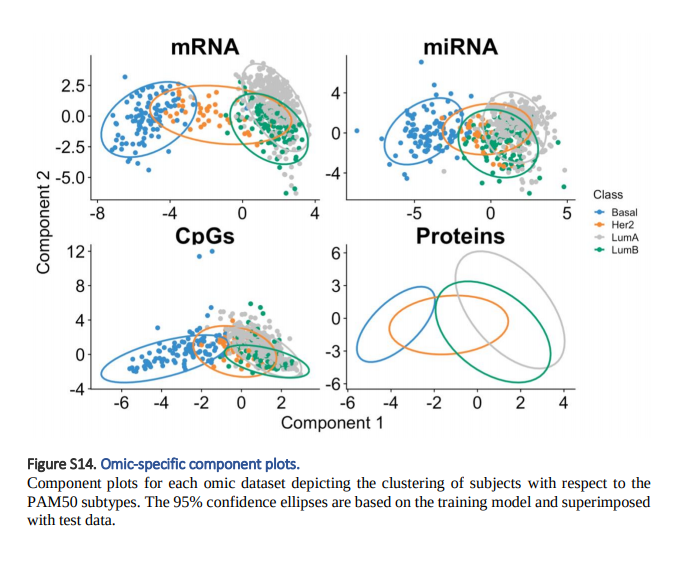
1. Sample Plots: Raw Data -> DIABLO -> Feature Embedding이 되었을 때, 각 Label 및 각 Omics별로 Clustering결과를 Visualization하여서 보여줍니다. 이러한 결과는 DIABLO Model이 각 Label에 따라 잘 분류를 실시할 수 있는지 보여주게 됩니다.

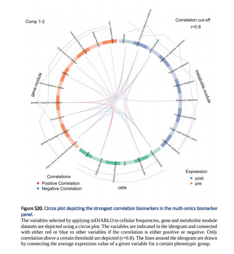
2. Variable Plots: Feature Selection상에서 각 선택된 변수와의 Correlation을 보여주는 Plot입니다. 이러한 Correlation은 Pearson Correlation으로서 슈사성 점수를 사용되어 계산됩니다.(Cut-off > 0.8) Line Plot은 각 표현형 그룹의 Expression입니다. => 즉, 각 변수별 Group간의 차이 및 다른 Omics와의 Correlation을 한번에 살펴볼 수 있습니다.

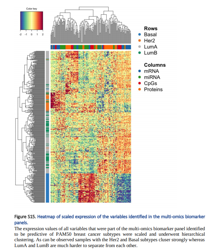
3. Clustered image mpas Plots: 각 Label 및 각 Omics별로 Expression을 Clustering하여 보여줍니다.

Simulation Dataset

많은 Experiments에서 사용되는 Simulation Dataset에 대하여 이해학고 있어야, Experiments의 결과가 이해되므로 어떠한 방식으로 Simulation Dataset을 만들었는지 확인한다.

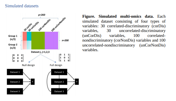
위의 Simulation Dataset은 다음과 같이 구성되어 있다고 한다.(위에 Simulation Figure 참조)

• Number of Dataset: 200(100: Group1, 100: Group2)
• Number of Features: 260
  • Correlated and discriminatory variables(corDis): 30
  • UnCorrelated and discriminatory variables(uncorDis): 30
  • Correlated and nondiscriminatory variables(corNonDis): 100
  • UnCorrelated and nondiscriminatory variables(uncorNonDis): 100
• Fold-Change(\(\triangle = \mu_{G2} - \mu_{G1} = [0, 1, 2]\)) => Fold Change의 값이 커질수록 두 Group간의 차이가 커진다.
• Covariance(\(\text{cov}(X_i, X_j) = [0, 5, 10, 15], \text{where } i\neq j\)) => Covaraiance의 값이 커질수록 Full design에서 상관있는 Feature를 많이 뽑아낸다.
• \(X_j = [X_j^{\text{corDis}} | X_j^{\text{uncorDis}} | X_j^{\text{corNonDis}} | X_j^{\text{uncorNonDis}} ] + E_j\)
  • \(E_j\): Error // Normal distribution with zero mean and variance equal to 0.2, 0.5, 1

Correlated and discriminatory variables(corDis)

$$X_j^{\text{corDis}} = \mu_j^{\text{corDis}}w_j^t \text{ ,where }\|w\|=1, j=1,2,3$$

• \(w_1, w_2, w_3\): Uniform Distribution in the interval of \([-0.3, 0.2] \cup [0.2, 0.3]\) with length 30
• \(\mu_1^{\text{corDis}}, \mu_2^{\text{corDis}}, \mu_3^{\text{corDis}}\): Multivariate normal distribution with a mean value of \(-\triangle/2(\triangle/2)\) with length 100 => Discriminatory
• \(\text{cov}(\mu_j^{\text{corDis}}, \mu_j^{\text{corDis}})=1 \text{, where }i,j=1,2,3, i\neq j\) => Correlated

UnCorrelated and discriminatory variables(uncorDis)

$$X_j^{\text{uncorDis}} = \mu_j^{\text{uncorDis}}w_j^t \text{ ,where }\|w\|=1, j=1,2,3$$

• \(w_1, w_2, w_3\): Uniform Distribution in the interval of \([-0.3, 0.2] \cup [0.2, 0.3]\) with length 30
• \(\mu_1^{\text{uncorDis}}, \mu_2^{\text{uncorDis}}, \mu_3^{\text{uncorDis}}\): Multivariate normal distribution with a mean value of \(-\triangle/2(\triangle/2)\) with length 100 => Discriminatory
• \(\text{cov}(\mu_j^{\text{uncorDis}}, \mu_j^{\text{uncorDis}})=0 \text{, where }i,j=1,2,3, i\neq j\) => UnCorrelated

Correlated and nondiscriminatory variables(corNonDis)

$$X_j^{\text{corNonDis}} = \mu_j^{\text{corNonDis}}w_j^t \text{ ,where }\|w\|=1, j=1,2,3$$

• \(w_1, w_2, w_3\): Uniform Distribution in the interval of \([-0.3, 0.2] \cup [0.2, 0.3]\) with length 30
• \(\mu_1^{\text{corNonDis}}, \mu_2^{\text{corNonDis}}, \mu_3^{\text{corDis}}\): Multivariate normal distribution with a mean value of 0 with length 100 => Non Discriminatory
• \(\text{cov}(\mu_j^{\text{corNonDis}}, \mu_j^{\text{corNonDis}})=1 \text{, where }i,j=1,2,3, i\neq j\) => Correlated

UnCorrelated and nondiscriminatory variables(uncorNonDis)

$$X_j^{\text{uncorNonDis}} = \mu_j^{\text{uncorNonDis}}w_j^t \text{ ,where }\|w\|=1, j=1,2,3$$

• \(w_1, w_2, w_3\): Uniform Distribution in the interval of \([-0.3, 0.2] \cup [0.2, 0.3]\) with length 30
• \(\mu_1^{\text{uncorNonDis}}, \mu_2^{\text{uncorNonDis}}, \mu_3^{\text{uncorNonDis}}\): Multivariate normal distribution with a mean value of 0 with length 100 => Non Discriminatory
• \(\text{cov}(\mu_j^{\text{uncorNonDis}}, \mu_j^{\text{uncorNonDis}})=0 \text{, where }i,j=1,2,3, i\neq j\) => UnCorrelated

Results

Correlation and discrimination tradeoff

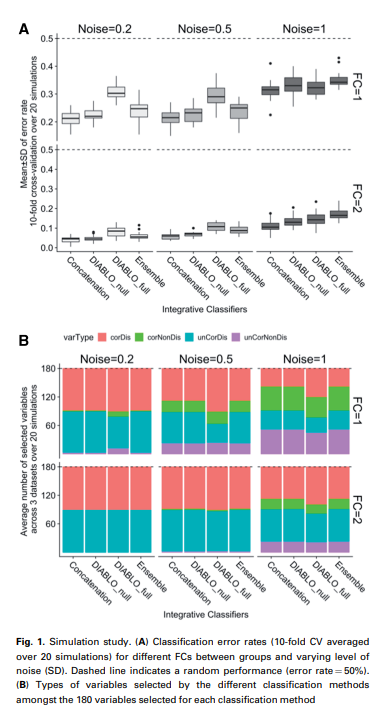
위의 Figure A는 Diablo의 결과와 다른 Model과의 차이를 보여주는 Figure이다. 해당 결과에서 주요하게 봐야 할 점은, Diablo_full의 경우에는 Classification결과에서는 다른 Model에서 좋은 성능을 보이지 않는다. 특히, Noise = 0.2 or 1인 경우에는 다른 Model보다 Error가 높은 것을 알 수 있다. 하지만 이러한 결과에 대해서 해당 논문은 다음과 같이 설명하고 있다.

We hypothesized that the increased error rate between the DIABLO models was due to the covariance constraint used to extract a common source of variation across datasets instead of independent sources of variation from each dataset.

따라서 Classification성능(discrimination) 뿐만 아니라 각각의 Modality의 Correlation을 얼마나 잘 고려하는지 또한 실험을 진행하였다. 위의 Figure B를 살펴보게 되면, DIABLO_full이 다른 Model들에 비하여 더 corDis + corNonDis Feature를 많이 선택한 것을 알 수 있다.

즉, 이러한 결과를 해당 논문에서는 Correlation and discrimination tradeoff라고 정의하고 있다.

Benchmark: DIABLO identifies highly interconnected networks with superior biological enrichment
Simulation Dataset이 아닌 실제 Real World Dataset을 사용하여 Experiment를 진행하게 위하여 아래와 같은 Dataset을 사용하였다.

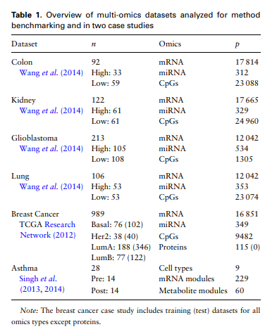
• Dataset: Colone, Kindney, Giloblastoma, Lung, Breast Cancer, Asthma
• Modality: mRNA, miRNA, CpGs
• Embedding Feature: 2
• Important Feature: 180(based on 90 variables with the largest weights on each of the 2 component)

주요하게 살펴봐야 할 Experiment Result는 2가지 이다.

1. Feature Selection

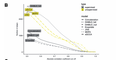
위의 결과를 살펴보게 되면 Unsupervised Method인 JIVE, sGCCA, MOFA는 Suprevised 방법에 비하여 많은 Edges를 찾는 것을 살펴볼 수 있다. 즉, Classification의 정보가 들어가지 않는 방법은 Modality간의 Correlation만 고려하므로, 당연한 결과라고 알 수 있다. 하지만, DIABLO_Full은 Classification의 정보가 들어감에도 불고하고, Unsupervised방법만큼 Modality끼리 관련된 Feature를 잘 찾는 것을 알 수 있다. 즉, Design Matrix에서 관계가 있다고 정의하면, 충분히 Classification + Feature Selection이 잘 되는 것을 알 수 있다.

2. Classification

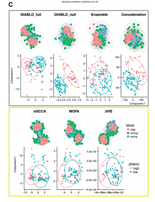
위의 결과를 살펴보게 되면 Unsupervised Method인 JIVE, sGCCA, MOFA는 Suprevised 방법은 눈으로 살펴보았을 경우 거의 Classification을 할 수 없게 Embedding하는 것을 알 수 있다. 하지만, Supervised Method의 Embedding은 Classification을 할 수 있게 Embedding이 되는 것을 알 수 있다. 주요하게 살펴봐야 할 점은 Visual상으로는 DIABLO_null이 가장 우수한 것을 알 수 있다.

즉, 각 Modality의 Correlation을 고려하면서 Classification의 성능이 높은 것은 DIABLO_FULL이다 라고 말할 수 있다. (Classification의 성능만 두고 보면 DIABLO_null이 가장 높고 이러한 이유로는 Modality간의 Correlation을 고려하지 않기 때문이다.)

Competitive performance and identification of known and novel multi-omics biomarkers of breast cancer subtypes
Hyperparameter Tuning을 포함하여 모든 Model의 결과를 직접 비교하였다. DIABLO_null, DIABLO_full은 Train Error: 19%, Test Error: 21%인 반면에 ENbsemble-based methods error는 Train Error: 11%, Test Error: 28%로서 Overfitting된 모습을 보여준다. 해당 결과에 대해서 해당 논문은 다음과 같이 설명하고 있다.

We noted that Concatenation-based classifiers tended to be biased towards the more predictive variables (mRNA or CpGs), whereas DIABLO selected variables evenly across datasets and had similar error rates between training and test datasets.

(위와 같은 결과를 얻기 위해서는 Dataset이 Train에서는 특정 Modality에서만 중요하고, Test에서는 모두 중요한 Sample을 Selection해야 된다는 가정이 있어야 된다. 실제 Dataset을 보지 않아서 맞는 Experiment결과인지는 알 수 없었다.)

Discussion

해당 논문은 Multi-Omics간의 Correlation이 높은 Feature Selection + Classification Model로서 장점과 단점을 모두 서술한 Paper였다.

특히 Correlation and discrimination tradeoff Experiment결과에서 알 수 있듯이, Correlation이 높게 설정하여 관련있는 Feature를 Selection하게 되는 경우, Classification의 성능을 떨어질 수 밖에 없는 Tradeoff가 발생한다. 이러한 결과는 당연한 결과인데 다른 논문들에서는 Classification도 잘되면서 Correlation이 높은 Feature또한 잘 선택할 수 있다고 서술하여 개인적으로는 객관성이 떨어져 보였으나, 해당 논문은 아니였다.

해당 논문 마지막에 결국 어쩔수 없이 Multi-Omics간의 Linear한 Relationship밖에 고려할 수 없다는 것을 단점으로 뽑았다. 개인적인 생각으로는 Non-Linear한 Model로 구성하게 되면, Classification의 성능을 오를 수 있으나, Non-Linear한 관계가 있는 Feature를 뽑았을 경우, 이러한 Feature가 서로 관계있다는 것은 알 수 없고, 단순히 Classification판단에 도움을 준다는 것이 한계일 것 같다.