Paper19. Sampling Matters in Deep Embedding Learning

Sampling Matters in Deep Embedding Learning

출처: Sampling Matters in Deep Embedding Learning
코드: suruoxi Github

Abstract

Deep embeddings answer one simple question: How similar are two images? Learning these embeddings is the bedrock of verification, zero-shot learning, and visual search. The most prominent approaches optimize a deep convolutional network with a suitable loss function, such as contrastive loss or triplet loss. While a rich line of work focuses solely on the loss functions, we show in this paper that selecting training examples plays an equally important role. We propose distance weighted sampling, which selects more informative and stable examples than traditional approaches. In addition, we show that a simple margin based loss is sufficient to outperform all other loss functions. We evaluate our approach on the Stanford Online Products, CAR196, and the CUB200-2011 datasets for image retrieval and clustering, and on the LFW dataset for face verification. Our method achieves state-of-the-art performance on all of them.

해당 논문에서 강조하고 있는 것은 단순히 Deep Embedding Learning(Metric Learning)에서 Loss도 중요하지만, Sampling또한 매우 중요하다고 강조하고 있다. 따라서, 간단한 Loss를 사용하여도 Sampling에 따라 State-Of-The-Art의 Performance를 보여줄 수 있다고 한다.

해당 논문은 이러한 Sampling을 “Distance weighted sampling”이라고 칭하고 있다. 기존의 Metric Learning인 Unsupervised Feature Learning via Non-Parametric Instance Discrimination, Beyond triplet loss: a deep quadruplet network for person re-identification, FaceNet: A Unified Embedding for Face Recognition and Clustering의 경우에는 Semi-Hard or 다른 간단한 Sampling방법을 소개하였지만, Sampling 방법에 따라 Performance는 비교하지 않았다. 해당 논문에서는 Sampling방법에 초점을 맞추고, 효과적이고 Stable하게 Training가능한 Sampling방법을 소개한다.

Introduction

먼저 Deep Embedding Learning의 과정을 살펴보면, 아래 Figure와 같다.

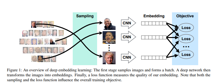
모든 Metric Learning의 Focus는 2가지로 나타낼 수 있다.

1. Similarity를 학습하는 Loss를 위하여, Dataset을 Pair로 잡아야 하기 때문에 Dataset을 어떻게 “Sampling”할 것인가?
2. Model을 학습할 Loss를 어떻게 구성할 것 인가?

많은, Model은 Loss를 어떻게 구성할 것인가에 초점을 두고, 그에 따른 Sampling방법을 많이 선택하게 된다. 하지만, 현재 논문에서는 다음과 같이 이야기 하고 있다.

In this paper, we show that sample selection in embedding learning plays an equal or more important role than the loss.

Sampling방법이 Loss보다 더 효과적이다 라는 것을 Experiments를 통하여 증명하고, 효과적인 Sampling방법에 대하여 설명한다. 또한 이러한 Loss는 Lower varance of gradients를 보장하여 Training이 Stable하다고 얘기하고 있다.

이러한 방식은 절대적인 Distance를 기반으로 이루워지는 것이 아니라 isotonic regression을 통하여 이루워진다고 하고 있다.

참조: Disadvantage of fix margin
해당 논문은 abolute distance를 사용하면 다음과 같은 단점이 있다고 얘기하고 있다.

However, using the same fixed distance for all images can be quite restrictive, discouraging any distortions in the embedding space.

해당 문제점에 대해서는 저도 같은 생각이였습니다. Beyond triplet loss: a deep quadruplet network for person re-identification에서는 Batch Dataset안의 Positive & Negative의 Distance의 평균으로서 Adaptive Margin을 적용하였습니다. 해당 논문은 Isontonic Regression을 통하여 해결하였다고 하고 있습니다.

참조: Isontonic Regression
Isontonic Regression은 Calibration Model중에 하나의 예시라고 나와있습니다. Model에 대한 Output뿐만 아니라 그러한 Output에 대한 Confidence까지 같이 계산하는 Model의 종류로서 알려져 있습니다. 망나 Blog는 이러한 Calibration Model에 대한 논문에 대한 Review가 자세히 적혀있습니다. (아직 정확히 읽어보지 않아서 정리하지는 않았습니다.)

또한 해당논문에서 이러한 Isontonic Regression을 사용하는 이유를 다음과 같이 설명하고 있습니다.

This plethora of loss functions is quite reminiscent of the ranking problem in information retrieval. There a combination of individual, pair-wise [14], and list-wise approaches [35] are used to maximize relevance. Of note is isotonic regression which disentangles the pairwise comparisons for greater computational efficiency. See [21] for an overview

• [21] IntervalRank — Isotonic Regression with Listwise and Pairwise Constraints

해당 논문은 읽어보지 않았으나, Isontonic Regression이 pairwise comparisons에서 computational efficiency가 있다고 설명하고 있습니다. 즉, Fix된 Margin이 아닌 Rank으로서 계산하기 위하여 사용한 것으로 생각됩니다.

Preliminaries

Notation

• \(x_i \in \mathbb{R}^N\): Data
• \(f: \mathbb{R}^N \rightarrow \mathbb{R}^D\): Deep network
• \(f(x_i)\): Latent Representation
• \(\| \cdot \|\): Euclidian Distance
• \(D_{ij} = \| f(x_i) - f(x_j)\|\): Distance between two datapoints
• \(y_{ij} \begin{cases} 1 & \text{Positive pair} \\ 0 & \text{Negative Pair} \end{cases}\): Label
• \(\alpha\): Margin

Contrast Loss

$$l^{\text{contrast}}(i,j) = y_{ij}D_{ij}^2 + (1-y_{ij})[\alpha - D_{ij}]^2_{+}$$

Triplet Loss

$$l^{\text{triplet}}(a,p,n) = [D_{ap}^2 - D_{an}^2 + \alpha]_{+}$$

Distance Weighted Margin-Based Loss

Abstract에서 언급하였듯이 Contrast Loss를 사용할 경우 \(O(n^2)\), Triplet Loss를 사용할 경우 \(O(n^3)\)의 Pair Dataset이 사용된다. 이러한 Dataset은 실질적으로 Computation infeasible하다. 따라서 Semi-Hard Sampling, Hard Sampling, Random Sampling, Uniform Sampling의 방법으로 Sampling을 실시하여 Dataset을 구축한다.
해당 논문은 이러한 대표적인 Sampling에 대한 단점을 설명하고 이를 해결하기 위한, Distance Weighted Sampling를 보여준다.

먼저, 중요하게 가정하고 가는 것은 Distance를 기준으로 Negative를 Sampling을 할때, Uniformly하게 Sampling이 가능하다는 것 이다.

해당 논문에서, 먼저 \(n\)-dimensional unit sphere \(\mathbb{S}^{n-1}, n\ge 128\)인 경우, Data points가 uniformly distributed on sphere라고 가정하면 다음과 같이 distribution of pairwise distance의 식을 나타내었다.

$$q(d) \propto d^{n-2}[1-\frac{1}{4}d^2]^{\frac{n-3}{2}}$$

이러한 식은 다음과 같이 Figure2로서 표현된다.

식은 어렵지만, 결국 Feature Embedding의 Output이 Normalization이 되어 나올 때, Output의 길이는 unit vector가 될 것이고, 따라서 Output은 Sphere형태를 띌 것이다. 모든 Dimension에서 Uniformly distribution이라면 위와 같은 식이 되는 것 이다.

이러한 식은 n이 충분히 크다면 \(N(\sqrt{2}, \frac{1}{2n})\)의 Normal Distribution의 형태로 나타낼 수 있는 것을 확인할 수 있다.

해당 논문의 Supplement중 아래 그림은 실제 훈련중에 Negative Distance Distribution을 보여준다.

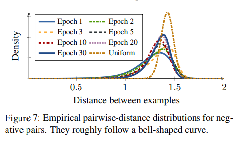
식에서 유도하였듯이, first epoch이후에는 distribution이 bell shape인것을 확인할 수 있고, epoch가 지나갈 수록 점차적으로 concentrates(분산이 작아지는)되는 결과를 확인할 수 있다.

Why not using hard sample

해당논문에서는 기존에 많이 사용하는 Semi-Hard, Hard를 사용하지 않고, Distance weighted sampling을 사용한다. 기존의 Semi-Hard, Hard Sampling의 단점을 알아보기 위하여 다음과 같은 식을 살펴보자.

$$\partial_{f(x_n)} l^{(\cdot)} = \frac{h_{an}}{\|h_{an}\|}w(t)$$

• \(h_{an} = f(x_a) - f(x_n)\)
• \(w(\cdot)\): Some Function

위의 식은 Negative sample Output에 대한 Triplet Loss Deviation이다. 위의 식을 살펴보게 되면 \(\frac{h_{an}}{\|h_{an}\|}\)은 Gradient의 Direction을 나타내는 것을 알 수 있다. 만약, enough noise를 \(z\)라 하면, Direction은 \(\frac{h_{an}+z}{\|h_{an}+z\|}\)가 될 것이다. 즉, Anchor와 Negative Sample간의 Distance인 \(h_{an} = f(x_a) - f(x_n)\)이 작아지면 작아질 수록, Noise에 영향을 많이 받는 것을 확인할 수 있다.

아래 Figure는 \(z \text{~} N(0, \sigma^2 U)\)에 대한 nuclear norm of covariance matrix를 Visualization한 결과이다.

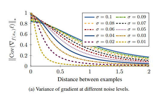
위의 결과를 확인하면, Distance가 작을수록, Noise와 Noise가 없는 Loss의 Covariance가 커지는 것을 확인할 수 있다. 즉, Hard Sample일 수록, Noise에 대한 Robust능력이 없어지게 되고 이로 인하여 Converge하는데 오랜 시간이 걸리거나 Training이 Stable하지 않다는 결과를 얻을 수 있다.

Distance wighted sampling

Distance Weighted Sampling의 식은 다음과 같다.

$$\text{Pr}(n^{\star}=n | a) \propto \text{min}(\lambda, q^{-1}(D_{an}))$$

위에서 언급한 Pairwise distance의 Inverse를 취하여 weight로서 sampling을 실시하게 된다. 즉, Dataset이 많은 부분은 weight를 적게, Dataset이 많은 부분에는 weight를 크게 하여, Distance 에 상관없이 uniformly하게 sampling이 가능하게 된다.

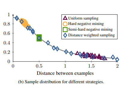
Distance weighted sampling과 다른 sampling방법의 차이는 아래 그림과 같다.

• Uniform sampling(=Random Samping): Density of datapoints on the D-dimensional unit sphere을 보게 되면 대부분의 sample은 \(\sqrt{2}\)에 집중되어있는 것을 알 수 있다. 따라서 Uniform한 weight로서 sampling을 하게 되면, 대부분의 sample의 distance는 \(\sqrt{2}\)가 될 것이고, 너무 쉬운 sample로서 학습을 하게 되므로 Loss=0이 된다.

• Hard negative mining: Hard negative sample로서 sampling을 실시하게 되면, 모든 sample이 Loss가 0이아닌 sample로서 학습할 sample이 많아지는 것을 확인할 수 있다. 하지만, “Why not using hard sample”에 설명한 단점을 그대로 가지는 sample만 사용하는 것을 알 수 있다.

• Semi-hard negative mining: 대부분의 다른 논문에서 사용하는 sampling방법이다.하지만, 위의 Figure에서도 알 수 있듯이, sample의 범위가 너무 narrow한 것을 살펴볼 수 있다. 즉, Training초기에는 효과적인 학습 방법이지만 어느 정도 진행됨에 따라서 학습이 진행되지 않고 Local Minimum에 수렴하는 것을 살펴볼 수 있다.

Margin based loss

Advantabes of Triplet Loss((\(l_2\)))
해당 논문에서는 또한 Margin based loss를 설명하고 있다. 이 Loss에 대해 알아보기 전에 기존의 Loss를 설명하는 Figure를 살펴보자.

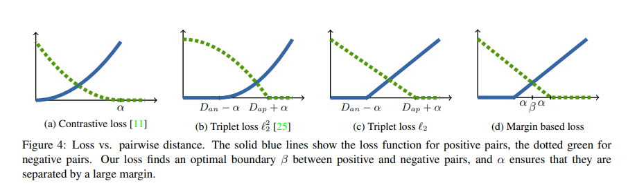
• (a): \(y_{ij}D_{ij}^2 + (1-y_{ij})[\alpha - D_{ij}]^2_{+}\)
• (b): \([\|f(x_a) - f(x_p)\|_2^2 - \| f(x_a) - f(x_n)\|_2^2 +\alpha]_{+}\)
• (c): \([\|f(x_a) - f(x_p)\|_2 - \| f(x_a) - f(x_n)\|_2 +\alpha]_{+}\)

위의 그림을 보게되면, Triplet Loss(b)가 Contrastive Loss(a)보다 좋은 점이 2개 있다고 논문에서 언급하고 있다.

1. Contrastive Loss는 \(\alpha\)라는 specific한 threshold를 지정하는 반면, Triplet Loss는 Similarity(\(D_{ap}\))와 Dissimilarity(\(D_{an}\))을 통하여 유연하게 학습이 가능하다. 이러한 결과로서 Intra Class간의 variation을 다르게(상대적으로)줄 수 있다.
2. Triplet Loss는 Anchor를 기준으로 Positive가 Negative에 비해 상대적으로 가깝게 유지시킨다. 하지만, Contrastive Loss는 모든 Positive Sample을 가깝게 Clustering하는 Loss이다. 즉, Overfitting의 위험이 있어 실생활에서는 잘 사용하지 않는 Loss이다.

또한 Trplet Loss(\(l_2^2\))의 문제점과 해결방안으로서 Triplet Loss(\(l_2\))에 대하여 설명하고 있다.
Triplet Loss(\(l_2^2\))의 경우에는 Negative Loss(Green Line)에 대해서는 Loss가 Concave하다. Hard Negative가 되면 될 수록, 특히 Gradient는 0에 가까워 진다. 하지만 이에비해 Hard Positive에 대해서는 Gradient가 매우커지는 것을 알 수 있다.
하지만, Triplet Loss((\(l_2\)))를 사용하는 경우에는 이러한 문제점을 모두 해결하는 것을 보여준다.

Margin based Loss
(자세히 이해하지 못하였습니다. 해당 논문의 본문을 보시는 것을 추천드립니다.)
해당 논문에서는 이러한 Triplet Loss((\(l_2\)))와 동일한 효과를 하는 Margin based Loss에 대해서 설명하고 있다.

$$l^{\text{margin}}(i,j) = (\alpha+y_{ij}(D_{ij}-\beta))_{+}$$

• \(\alpha\): Margin
• \(y_{ij} \in \{-1, 1\}\)

위의 Loss를 살펴보게 되면 Contrastive Loss와 같이 Computation Cost는 얼마 들지 않고(Dataset이 Pair로 들어가게 되므로), Triplet Loss(\(l_2\))와 같은 효과를 낼 수 있는 것을 확인할 수 있다.

하지만, \(\beta\)를 정의해야되는데, 단순한 Constant로 정의하면, Contrastive Loss와 동일하게 되는 것을 알 수 있다. 따라서 해당 논문은 \(\beta\)를 Positive와 Negative pair의 boundary정의할 수 있는 Variable로서 정의하게 된다.

$$\beta = \beta^{(0)} + \beta_{c(i)}^{\text{class}} + \beta_{i}^{img}$$

• \(\beta\): flexible boundary parameter
• \(\beta_{c(i)}^{\text{class}}\): Class specific
• \(\beta_{i}^{img}\): Example specific

해당 논문에서는 \(\beta\)를 단순히 어떠한 값이 아니라, class와 example을 고려하여 정한다고 나와있다. (자세히 어떻게 정의하는지, 그 값을 어떻게 Update하는지에 대해서는 잘 나와있지 않다.)

해당 \(\beta\)와 regularization을 가하면 다음과 같은 최종적인 Loss를 얻을 수 있다.

$$\partial_{\beta} l^{\text{margin}}(i,j) = -y_{ij} 1 \{\alpha > y_{ij}(\beta - D_{ij})\}$$

$$\text{minimize} \sum_{(i,j)} l^{\text{margin}}(i,j) + v(\beta^{(0)} + \beta_{c(i)}^{(\text{class})}+\beta_{i}^{\text{img}})$$

Experiments

Setting

• Dataset: CARD196, CUB200-2011, Stanford Online Products
• Input: 224 x 224 // Embedding: 128
• \(\alpha = 0.2, \beta^{0} = 1.2, \beta^{\text{class}} = \beta^{\text{img}} = 0\): Margin Fix, \(\beta\) Initialize

Effect of Sampling

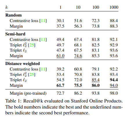
위의 결과는, Loss는 동일하게 학습하되 Sampling의 방법만 바꾸고 실험한 결과이다. 기본적으로 많이 사용하는 Random과 Semi-Hard Sampling과 해당 논문에서 주장하는 Distance weighted Sampling을 비교한다. 중요하게 봐야할 결과는 Loss에 상관없이 Distance weighted Sampling을 사용하는 것이 Performance가 좋은 것을 살펴볼 수 있다. 또한 “Margin based loss”에서 보았듯이 Contrastive Loss < Triplet Loss(\(l_2^2\)) < Triplet Loss(\(l_2\)) < Margin Loss순으로 Performance가 좋은 것을 알 수 있다.

Convergence speed

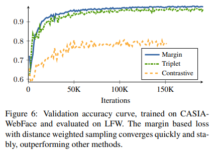
• Margin Loss + Distance Weighted Sampling
• Triplet Loss + Semi-Hard Sampling
• Contrastive Loss + Random Sampling

위의 결과를 확인하게 되면, Margin Loss + Distance Weighted Sampling이 빠르게 수렴하고 Performance도 좋은 것을 알 수 있다. Semi-Hard Sampling또한 Performance가 좋으나, 수렴하기까지 오래 걸리는 것을 알 수 있다.

Quantitative Results
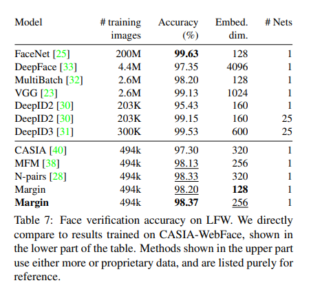해당 결과를 보게 되면, Training Images가 동일한 다른 Model에 비하여 Embedding Dimension이 작음에도 불고하고 Performance가 높은 것을 확인할 수 있다.

Conclusion

해당 논문의 Contribution은 다음과 같다고 생각한다.

1. 기존의 Metric Learning의 논문들과 달리 Loss에 중점을 맞춘 것이 아닌 범용적으로 사용할 수 있는 새로운 Distance weighted sampling을 제시하였다. 또한, 이러한 sampling방법과 비교하여 기존의 sampling방법들의 단점을 명확히 설명하고 있다.
2. Metric Learning에서 많이 사용하는 Contrastive learning, Triplet Loss에 대한 단점을 명확히 지적하고 차이점을 설명하였다. 또한 각각의 방법에서 장점을 사용하는 Margin-Based Learning에 대해서 설명하고 있다.

Margin-Based Learning에 대해서는 정확히 나와있는 Code가 없는 듯 한다. 정확한 \(\beta^{\text{class}}_{c(i)}, \beta_i^{text{img}}\)에 대하여 Update방식이나, 어떻게 지정해야 되는지 모르겠어서 Code화를 하는 것이 아쉽다.

하지만, Distance weighted Sampling은 Code가 있고 이러한 Sampling방법은 다른 Sampling방법들 보다 좋은 방법이라고 생각된다.

Pytorch Code

출처: suruoxi Github

get_distance

• \(x \in R^{N \times F}, \|x\| = 1\): Input(L2 Normalization Input)
• \(\text{dist} \in R^{N \times N}\): Output(Distance between Samples)

아래 Function은 Euclidian Distance이다. Wikipedia

$$|A-B|^2 = (A-B)^T(A-B) = |A|^2 + |B|^2 - 2A^TB$$

$$ = 2(1-\text{cos}(A,B)) (\text{ s.t.}|A| = |B| = 1)$$

def get_distance(x):
    _x = x.detach()
    sim = torch.matmul(_x, _x.t())
    dist = 2 - 2*sim
    dist += torch.eye(dist.shape[0]).to(dist.device)   # maybe dist += torch.eye(dist.shape[0]).to(dist.device)*1e-8
    dist = dist.sqrt()
    return dist

DistanceWeightedSampling
아래 Code에서 중요한 부분은 다음과 같다.

log_weights = ((2.0 - float(d)) * distance.log() - (float(d-3)/2)torch.log(torch.clamp(1.0 - 0.25(distance*distance), min=1e-8))) = \((2-n)\text{log}(d) + \frac{3-n}{2}\text{log}(1-\frac{1}{4}d^2) \propto \text{log}(q(d)^{-1})\)

• distance: Distance
• d: Embedding Dimension

class   DistanceWeightedSampling(nn.Module):
    '''
    parameters
    ----------
    batch_k: int
        number of images per class
    Inputs:
        data: input tensor with shapeee (batch_size, edbed_dim)
            Here we assume the consecutive batch_k examples are of the same class.
            For example, if batch_k = 5, the first 5 examples belong to the same class,
            6th-10th examples belong to another class, etc.
    Outputs:
        a_indices: indicess of anchors
        x[a_indices]
        x[p_indices]
        x[n_indices]
        xxx
    '''

    def __init__(self, batch_k, cutoff=0.5, nonzero_loss_cutoff=1.4, normalize =False,  **kwargs):
        super(DistanceWeightedSampling,self).__init__()
        self.batch_k = batch_k
        self.cutoff = cutoff
        self.nonzero_loss_cutoff = nonzero_loss_cutoff
        self.normalize = normalize

    def forward(self, x):
        k = self.batch_k
        n, d = x.shape
        distance = get_distance(x)
        distance = distance.clamp(min=self.cutoff)
        log_weights = ((2.0 - float(d)) * distance.log() - (float(d-3)/2)*torch.log(torch.clamp(1.0 - 0.25*(distance*distance), min=1e-8)))

        if self.normalize:
            log_weights = (log_weights - log_weights.min()) / (log_weights.max() - log_weights.min() + 1e-8)

        weights = torch.exp(log_weights - torch.max(log_weights))

        if x.device != weights.device:
            weights = weights.to(x.device)

        mask = torch.ones_like(weights)
        for i in range(0,n,k):
            mask[i:i+k, i:i+k] = 0

        mask_uniform_probs = mask.double() *(1.0/(n-k))

        weights = weights*mask*((distance < self.nonzero_loss_cutoff).float()) + 1e-8
        weights_sum = torch.sum(weights, dim=1, keepdim=True)
        weights = weights / weights_sum

        a_indices = []
        p_indices = []
        n_indices = []

        np_weights = weights.cpu().numpy()
        for i in range(n):
            block_idx = i // k

            if weights_sum[i] != 0:
                n_indices +=  np.random.choice(n, k-1, p=np_weights[i]).tolist()
            else:
                n_indices +=  np.random.choice(n, k-1, p=mask_uniform_probs[i]).tolist()
            for j in range(block_idx * k, (block_idx + 1)*k):
                if j != i:
                    a_indices.append(i)
                    p_indices.append(j)

        return  a_indices, x[a_indices], x[p_indices], x[n_indices], x

---

참조: Sampling Matters in Deep Embedding Learning
참조: sooooojinlee GitHub

코드에 문제가 있거나 궁금한 점이 있으면 wjddyd66@naver.com으로 Mail을 남겨주세요.