Tensorflow-FCN

Segmentation

먼저 Image에대해서 판단하는 방법들에 대해서 알아보자.
아래 그림을 살펴보면 Image를 판단하는 문제를 크게 3가지의 문제로 잘 분류하였다.

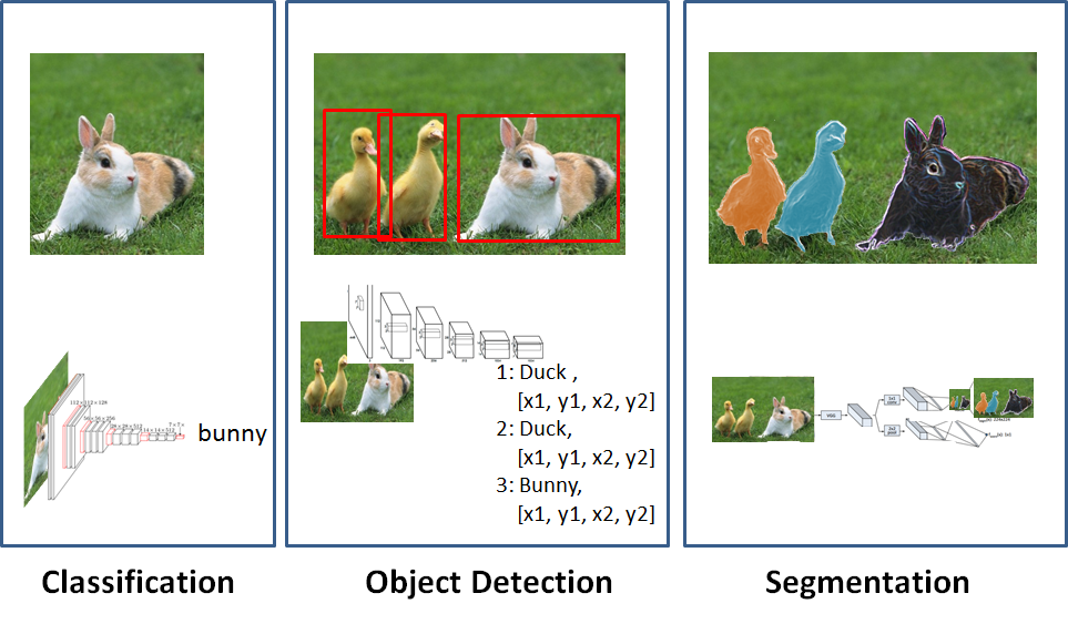
그림 출처: ataspinar.com
위의 그림을 살펴보면 각각을 다음과 같이 분류하였다.

• Classification: 사진안의 Object를 어떤것인지 판단하는 이미지 분류 방법
• Object Detection: 사진안의 각각의 Object를 어떤것인지 판단하는 이미지 분류 방법
• Segmentation: 사진안의 각각의 Object를 위치와 Object에 따라서 색을 달리하는 이미지 분류 방법

즉 ,Segmentation은 Object의 대략적인 위치가 아닌 정확한 위치와 Classification을 정확히 하여 나타내는 방법이기 때문에 Object Detection보다 좀 더 어려운 이미지 분류 방법으로 평가 받는다.

이러한 Segmentation은 두가지로 나뉘게 된다.

• Semantic Segmentation: 각각의 Object가 어떤 class인지만을 구분
• Instance Segmentation: 같은 Class이더라도 다른 것이라면 구분하는 문제

그림 출처: sualab.com
이러한 Segmentation에 따라서 Data전처리 과정에서 어떻게 Maskin할지가 달라기고 공통적인 Algorithm은 같다.

FCN

참조 논문: Fully Convolutional Networks for Semantic Segmentation
FCN이란 Fully Convolution Network의 약자로서 Network의 모든 Layer를 Convolution으로 구성하였다는 것 이다.
FCN의 Network 구조를 살펴보면 다음과 같다.

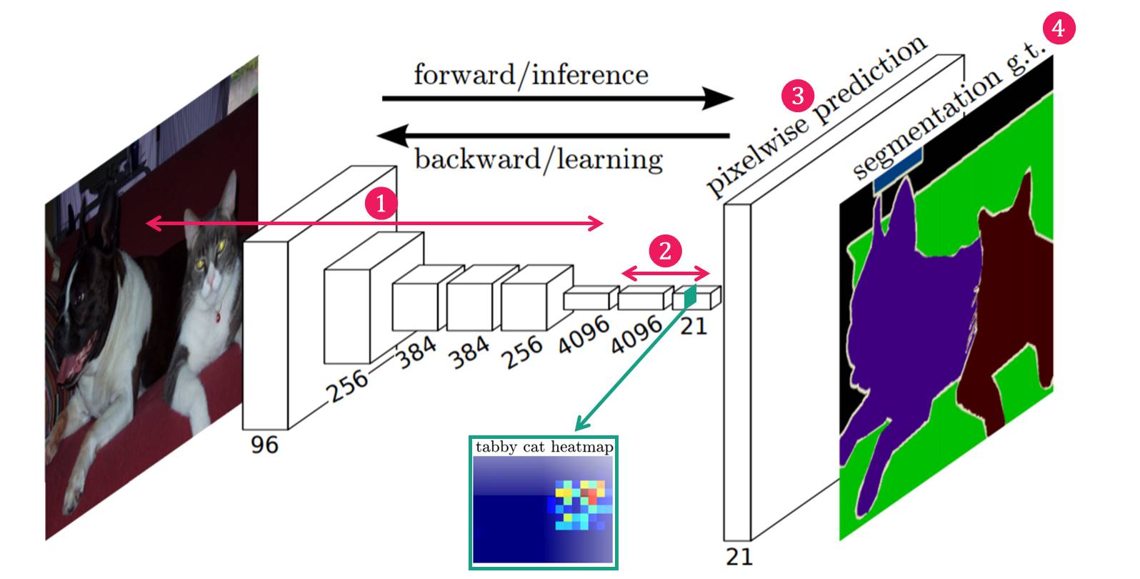
사진 출처: modulabs-biomedical 블로그
Network의 구조는 크게 4가지로 구분될 수 있다.

1. Feature Extraction: 일반적인 CNN Model에서 살펴볼 수 있는 Network의 구조로서 Image에서 Kernel과의 Convolution을 통하여 Image의 Feature를 뽑아내는 단계이다.
2. Feature-level Classification: 추출된 Feature map의 pixel하나하나마다 classification을 수행한다. Classification의 결과는 coarse하다. Feature map의 Dimension이 21인 이유는 Background(1) + Image Class(20)개로 나눈다는 의미이다.
3. Upsampling: coarse한 결과를 backward strided convolution을 통해 Upsampling하여 원래의 image size로 키워준다. 즉, Segmentation의 목적은 원래 크기의 Image를 Object별로 Class를 분류하는 것 이기 때문에 너무 Coarse한 Feature Map을 원래 크기의 Image를 키우면 정확한 결과가 나오지 않는다는 것 이다.
4. Segmentation: 각 Class의 Upsampling된 결과를 사용하여 하나의 segmantation결과 이미지를 만들어 준다.

Feature Extraction

Feature Extraction을 위하여 논문은 VGGNet을 사용하여 Feature Extraction을 수행하였다.

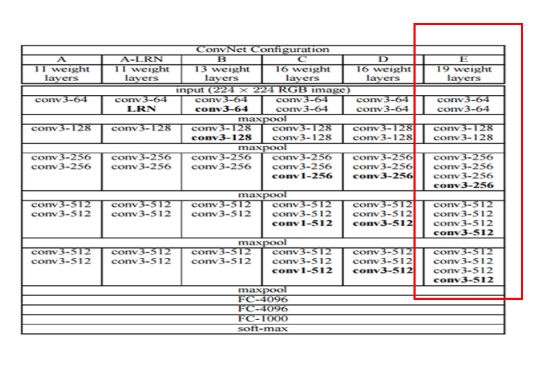
VGG는 위와같은 Layer 중 위에서 표시한 Box의 부분만을 사용하여 Feature Extraction을 수행하였다.
주의해야하는 점은 FC Layer를 Network의 구성요소로 사용하지 않았다는 것 이다.

Feature-level Classification

위에서 FCN은 FCN이란 Fully Convolution Network의 약자라고 선언하였다.
또한 위에서 VGG 를사용하여 FineTuning을 실시하지만 FC Layer는 거치지 않는다고 하였다.
즉, FCN은 VGG의 FC Layer를 Convolution으로 대체하였다고 할 수 있다.
사용한 Convolution은 1x1 Size의 Kernel을 이용하여 Convolution을 수행하였다.

먼저 FC Layer를 거치는 Image를 살펴보자

사진 출처: bskyvision.com

최종적인 결과는 1 Dimension의 1차원 Vector로서 나오게 된다. 이러한 결과는 Segmentation에서 중요한 위치정보를 잃게되는 불상사가 발생하게 된다. 이러한 FC Layer는 위에서 이미지 분류 중 Classification에서 사용한다.


다음으로 FC Layer를 1x1 Convolution으로 대체한 FCN을 살펴보자

사진 출처: bskyvision.com

위의 결과로서 알 수 있는 FCN의 장점을 살펴보자.

1. Image의 크기는 결국에 H/32 x W/32로서 Input Image의 크기는 상관이 없다. 기존의 Classification을 위해 FC Layer를 거쳐야하는 VGG Model은 Input Image의 크기를 일일이 맞춰줬어야 한다.
2. Feature Map은 H/32 x W/32라는 것은 Feature Map의 한 pixel은 Image의 32 x 32의 Feature를 대략적으로 가지고 있다고 할 수 있다.
3. 최종적인 결과로서 H/32 x W/32 x 21 의 결과를 얻을 수 있고 H/32 x W/32를 Heatmap(Feature map)이라고 칭한다. 이러한 Heatmap의 개수는 Image의 Class의 개수와 동일하다.(논문의 경우 Background(1) + Object Class(20) = 21) 이러한 Heatmap 21개는 각각의 Class를 대표한다. 예를들어 강아지 클래스에 대한 Heatmap이라면 강아지 위치의 Pixel값들이 높다.

Upsampling & Segmentation

Upsampling이란 Feature-level Classification를 통하여 H/32 x W/32 x 21의 Feature와 Location의 정보를 가지고 있는 Vector를 다시 원래의 Imae의 크기로 맞춰주어서 Segmentation을 하기위한 과정이다.
중요한 점은 Feature-level Classification의 결과가 Coarse한 결과라는 것이다.
즉, Heatmap의 한 pixel은 원본 Image의 32 x 32의 특징을 대략적(coarse)으로 가지고 있기 때문에 Upsampling결과 Detail한 Segemntation이 불가능하다는 것 이다.

이러한 점은 OpenCV의 디스크립터들이 가지는 문제와도 같다.
대표적인 이러한 문제점을 해결하는 방식은 이미지 피라미드를 구성하는 것 이다.
즉, 다양한 Image의 Size에서 Image의 전체적인 특징 부터 Detail한 특징까지 모두 합치는 과정이 필요하다.
참고로, Style Transfer에서도 Style Reconsturction과정에서 전체적인 분위기서부터 좁은 영역의 모든 분위기를 사용하기 위하여 위와 같은 과정을 사용하였다.
또한 Unet에서도 Copy and Crop의 과정에서 이러한 과정을 거쳤다.
즉, End to End Netowork의 구조에서 Feature Extraction결과에서 다시 Upsampling을 하는 Network의 구조에서는 위와 같은 과정이 필수인 것을 알 수 있다.

참고(Upsampling)
CNN에서 Upsampling의 경우 Deconvolution을 통하여 이루워 집니다. Deconvolution의 자세한 내용은 아래 링크를 참조하시기 바랍니다.
Deconvolution: Pytorch-Autoencoder

위와 같은 과정의 최종적인 결과는 아래 그림과 같다.

사진 출처: bskyvision.com

논문에서는 위의 그림의 최종적인 결과 Ground truth을 skip combining이라는 기법을 사용하여 구현하였다.


먼저 FCN-32s라고 표현한 결과부터 살펴보자.

사진 출처: bskyvision.com
FCN-32s는 위의 결과처럼 Heatmap의 크기를 단순히 32배로 증가시키는 과정으로 이루워졌다.
앞에서도 이야기 하였지만 Heatmap은 Coarse한 특성이므로 전체적인 Detail을 표현하기에는 부족하다는 것을 알 수 있다.


FCN-16s라고 표현한 결과를 살펴보자.

사진 출처: bskyvision.com
최종적인 Heatmap을 얻기 전의 결과 Pool4(Feature map)과 최종적인 결과 Conv7(Heatmap)을 더하여 Deconvolution과정을 통하여 Upsampling하는 과정이다.
여기서 Pool4와 Conv7의 Size가 맞지 않으므로 다음과 같은 과정을 거치게 된다.

1. Conv7 x 2Upsampling = Conv7-2
2. Pool4 + Conv7-2 = Result2
3. Result2 x 16Upsampling

위와 같은 과정으로 Coarse한 특성을 좀 더 완만하게 해결하였다.


FCN-8s라고 표현한 결과를 살펴보자.

사진 출처: bskyvision.com
FCN-16s와 같이 각각의 Feature Map의 Size를 맞춘 뒤 합쳐서 Upsampling을 하는 것을 알 수 있다.
최종적인 Target Image인 Ground truth에 비교하였을때 FCN-32s -> FCN-16s -> FCN-8s로 갈수록 점점 Detail하게 Segmentation의 결과를 얻을 수 있는것을 확인할 수 있다.

FCN 구현

원본 Code는 shekkizh GitHub입니다.
Code의 구성은 다음과 같습니다.

• FCN.py: Trainning, Evaluation, Model, Test를 진행하는 Code
• BatchDatasetReader.py: Trainning을 위하여 Dataset을 Batch로 바꿔주는 역할
• TensorflowUtil.py: Trainning된 VGGModel과 VGGModel에서 사용할 일부 Network, Image처리 등을 위하여 Utility를 모아둔 Code
• read_MITSceneParsingData.py: 실질적인 Data를 다운받고 Data를 원하는 Name으로 바꾸는 Code
• result_color_visualization.ipynb: 최종적인 결과를 Color Image로 바꾸어서 확인하는 Code

FCN.py를 제외한 Utility의 함수의 경우 모두 주석으로 설명이 매우 잘 되어있습니다.
또한 Code의 길이가 매우 길어서 제일 중요한 FCN.py에 대해서만 설명하겠다.

FCN.py
필요한 라이브러리 Import
기본적인 tensorflow, numpy뿐만아니라 Trainning과 Utility를 포함한 Python File까지 모두 import한다.

from __future__ import print_function
import tensorflow as tf
import numpy as np
import datetime

import TensorflowUtils as utils
import read_MITSceneParsingData as scene_parsing
import BatchDatsetReader as dataset

학습에 필요한 Parameter를 tf.flag.FLAGS API를 이용하여 지정한다.

FLAG	설명
batch_size	Batch size
logs_dir	Tensorboard log를 지정할 경로
data_dir	Trainning, Validation에 필요한 Data의 경로
learning_rate	Learning Rate
model_dir	VGG Model Parameter가 지정된 mat File 경로
mode	Train 혹은 시각화인지 판단

# 학습에 필요한 설정값들을 tf.flag.FLAGS로 지정합니다.
FLAGS = tf.flags.FLAGS
tf.flags.DEFINE_integer("batch_size", "2", "batch size for training")
tf.flags.DEFINE_string("logs_dir", "logs/", "path to logs directory")
tf.flags.DEFINE_string("data_dir", "Data_zoo/MIT_SceneParsing/", "path to dataset")
tf.flags.DEFINE_float("learning_rate", "5e-5", "Learning rate for Adam Optimizer")
tf.flags.DEFINE_string("model_dir", "Model_zoo/", "Path to vgg model mat")
tf.flags.DEFINE_string('mode', "train", "Mode train/ visualize")

VGG Model Parameter
VGG-19 Parameter가 지정된 mat file의 URL과 Trainning에 필요한 Parameter 설정

• NUM_OF_CLASSESS = 151인 것을 보아 Dataset의 Class는 150개 + Background(1)로 Labeling된 것을 알 수 있다.
• INAGE_SIZE: VGG Model의 Input Size의 크기는 224이다.

# VGG-19의 파라미터가 저장된 mat 파일(MATLAB 파일)을 받아올 경로를 지정합니다.
MODEL_URL = 'http://www.vlfeat.org/matconvnet/models/beta16/imagenet-vgg-verydeep-19.mat'

# 학습에 필요한 설정값들을 지정합니다. 
MAX_ITERATION = int(100000 + 1)
NUM_OF_CLASSESS = 151       # 레이블 개수
IMAGE_SIZE = 224

VGG Model 정의
mat File로부터 Tensorflow로 API를 이용하여 VGGNet 그래프를 구축
먼저 TensorflowUtils.py에서 선언한 Method부터 살펴보자.

def get_variable(weights, name):
    init = tf.constant_initializer(weights, dtype=tf.float32)
    var = tf.get_variable(name=name, initializer=init,  shape=weights.shape)
    return var
    
def conv2d_basic(x, W, bias):
    conv = tf.nn.conv2d(x, W, strides=[1, 1, 1, 1], padding="SAME")
    return tf.nn.bias_add(conv, bias)
    
def avg_pool_2x2(x):
    return tf.nn.avg_pool(x, ksize=[1, 2, 2, 1], strides=[1, 2, 2, 1], padding="SAME")

위의 Method 각각은 다음과 같다.

• get_variable: Tensorflow의 Variable형태로 변환
• conv2d_basic: Convolution을 통하여 비선형 증가
• avg_pool_2x2: Pooling을 통하여 Image의 크기 1/2로 줄임

이제 위의 Method를 활용하여 실질적인 VGGNet구조를 살펴보자.

# VGGNet 그래프 구조를 구축합니다.
def vgg_net(weights, image):
  layers = (
    'conv1_1', 'relu1_1', 'conv1_2', 'relu1_2', 'pool1',

    'conv2_1', 'relu2_1', 'conv2_2', 'relu2_2', 'pool2',

    'conv3_1', 'relu3_1', 'conv3_2', 'relu3_2', 'conv3_3',
    'relu3_3', 'conv3_4', 'relu3_4', 'pool3',

    'conv4_1', 'relu4_1', 'conv4_2', 'relu4_2', 'conv4_3',
    'relu4_3', 'conv4_4', 'relu4_4', 'pool4',

    'conv5_1', 'relu5_1', 'conv5_2', 'relu5_2', 'conv5_3',
    'relu5_3', 'conv5_4', 'relu5_4'
  )

  net = {}
  current = image
  for i, name in enumerate(layers):
    kind = name[:4]
    # Convolution 레이어일 경우
    if kind == 'conv':
      kernels, bias = weights[i][0][0][0][0]
      # matconvnet: weights are [width, height, in_channels, out_channels]
      # tensorflow: weights are [height, width, in_channels, out_channels]
      # MATLAB 파일의 행렬 순서를 tensorflow 행렬의 순서로 변환합니다.
      kernels = utils.get_variable(np.transpose(kernels, (1, 0, 2, 3)), name=name + "_w")
      bias = utils.get_variable(bias.reshape(-1), name=name + "_b")
      current = utils.conv2d_basic(current, kernels, bias)
    # Activation 레이어일 경우
    elif kind == 'relu':
      current = tf.nn.relu(current, name=name)
    # Pooling 레이어일 경우
    elif kind == 'pool':
      current = utils.avg_pool_2x2(current)
    net[name] = current

  return net

위에서 조심해야 하는 점은 matconvnet과 tensorflow의 각각의 변수의 위치가 다르다는 것 이다.
VGGNet Model의 구조는 당연히 FC Layer가 포함되지 않았고 또한 중요한 점은 최종적인 Heatmap을 얻기 위해 pool 계층을 거치지 않았다는 것 이다.

FCN Model
위에서 선언한 VGGModel을 활용하여 FCN Model을 완성한다.

• image: input image
• keep_prop: drop out하지 않을 Node의 비율

# FCN 그래프 구조를 정의합니다.
def inference(image, keep_prob):
  """
  FCN 그래프 구조 정의
  arguments:
    image: 인풋 이미지 0-255 사이의 값을 가지고 있어야합니다.
    keep_prob: 드롭아웃에서 드롭하지 않을 노드의 비율
  """
  # 다운로드 받은 VGGNet을 불러옵니다.
  print("setting up vgg initialized conv layers ...")
  model_data = utils.get_model_data(FLAGS.model_dir, MODEL_URL)

  mean = model_data['normalization'][0][0][0]
  mean_pixel = np.mean(mean, axis=(0, 1))

  weights = np.squeeze(model_data['layers'])

  # 이미지에 Mean Normalization을 수행합니다.
  processed_image = utils.process_image(image, mean_pixel)

  with tf.variable_scope("inference"):
    image_net = vgg_net(weights, processed_image)
    # VGGNet의 conv5(conv5_3) 레이어를 불러옵니다.
    conv_final_layer = image_net["conv5_3"]

    # pool5를 정의합니다. 
    pool5 = utils.max_pool_2x2(conv_final_layer)

    # conv6을 정의합니다.
    W6 = utils.weight_variable([7, 7, 512, 4096], name="W6")
    b6 = utils.bias_variable([4096], name="b6")
    conv6 = utils.conv2d_basic(pool5, W6, b6)
    relu6 = tf.nn.relu(conv6, name="relu6")
    relu_dropout6 = tf.nn.dropout(relu6, keep_prob=keep_prob)

    # conv7을 정의합니다. (1x1 conv)
    W7 = utils.weight_variable([1, 1, 4096, 4096], name="W7")
    b7 = utils.bias_variable([4096], name="b7")
    conv7 = utils.conv2d_basic(relu_dropout6, W7, b7)
    relu7 = tf.nn.relu(conv7, name="relu7")
    relu_dropout7 = tf.nn.dropout(relu7, keep_prob=keep_prob)

    # conv8을 정의합니다. (1x1 conv)
    W8 = utils.weight_variable([1, 1, 4096, NUM_OF_CLASSESS], name="W8")
    b8 = utils.bias_variable([NUM_OF_CLASSESS], name="b8")
    conv8 = utils.conv2d_basic(relu_dropout7, W8, b8)

    # FCN-8s를 위한 Skip Layers Fusion을 설정합니다. 
    # 이제 원본 이미지 크기로 Upsampling하기 위한 deconv 레이어를 정의합니다.
    deconv_shape1 = image_net["pool4"].get_shape()
    W_t1 = utils.weight_variable([4, 4, deconv_shape1[3].value, NUM_OF_CLASSESS], name="W_t1")
    b_t1 = utils.bias_variable([deconv_shape1[3].value], name="b_t1")
    # conv8의 이미지를 2배 확대합니다.
    conv_t1 = utils.conv2d_transpose_strided(conv8, W_t1, b_t1, output_shape=tf.shape(image_net["pool4"]))
    # 2x conv8과 pool4를 더해 fuse_1 이미지를 만듭니다.
    fuse_1 = tf.add(conv_t1, image_net["pool4"], name="fuse_1")

    deconv_shape2 = image_net["pool3"].get_shape()
    W_t2 = utils.weight_variable([4, 4, deconv_shape2[3].value, deconv_shape1[3].value], name="W_t2")
    b_t2 = utils.bias_variable([deconv_shape2[3].value], name="b_t2")
    # fuse_1 이미지를 2배 확대합니다.
    conv_t2 = utils.conv2d_transpose_strided(fuse_1, W_t2, b_t2, output_shape=tf.shape(image_net["pool3"]))
    # 2x fuse_1과 pool3를 더해 fuse_2 이미지를 만듭니다.
    fuse_2 = tf.add(conv_t2, image_net["pool3"], name="fuse_2")

    shape = tf.shape(image)
    deconv_shape3 = tf.stack([shape[0], shape[1], shape[2], NUM_OF_CLASSESS])
    W_t3 = utils.weight_variable([16, 16, NUM_OF_CLASSESS, deconv_shape2[3].value], name="W_t3")
    b_t3 = utils.bias_variable([NUM_OF_CLASSESS], name="b_t3")        
    # fuse_2 이미지를 8배 확대합니다.
    conv_t3 = utils.conv2d_transpose_strided(fuse_2, W_t3, b_t3, output_shape=deconv_shape3, stride=8)

    # 최종 prediction 결과를 결정하기 위해 마지막 activation들 중에서 argmax로 최대값을 가진 activation을 추출합니다.
    annotation_pred = tf.argmax(conv_t3, dimension=3, name="prediction")

  return tf.expand_dims(annotation_pred, dim=3), conv_t3

위의 코드가 길지만 하나하나 살펴보면 다음과 같다.
먼저 def process_image(image, mean_pixel)을통하여 Image를 Mean Normalization한다.
def process_image()는 다음과 같이 정의된다.

def process_image(image, mean_pixel):
    return image - mean_pixel

다음으로 Normalization된 Image를 VGG Model을 거친뒤 Pooling을 하여 최종적인 Result를 얻게 된다.
pool5 = utils.max_pool_2x2(conv_final_layer): 이러한 과정으로 인하여 논문과 같이 원본이미지를 32배로 축소시켜 Feature Extraction과정을 거치는 것을 알 수 있다.
한가지 더 확인해야 하는 사실은 그 다음 conv6이다.
W6 = utils.weight_variable([7, 7, 512, 4096], name="W6"): 을 통하여 알 수 있는 사실은 \(224/2^5 = 32\)을 통하여 Input Image의 Size는 224 x 224 x channel 이라는 것 이다.

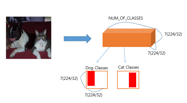
마지막으로 Heatmap을 얻기 위하여 최종적인 Vector를 위에서 선언한 NUM_OF_CLASSES의 Dimension으로 바꾼다.
W8 = utils.weight_variable([1, 1, 4096, NUM_OF_CLASSESS], name="W8"): 을 통하여 이제 각각의 W/32 x H/32 Image는 Classes에 포함되는 Pixel값이 높은 NUM_OF_CLASSES의 Dimension으로 이루워진 Vector를 얻을 수 있다.
그림으로 나타내면 아래와 같다.

이제 위에서 설명한 FCN-8s를 구현하기 위하여 Heatmap과 Featuremap의 Deconvolution을 통하여 합치는 과정을 진행한다.

1. HeatMap(conv8) 2배 확대: conv_t1 = utils.conv2d_transpose_strided(conv8, W_t1, b_t1, output_shape=tf.shape(image_net["pool4"]))
2. Pool4 + HeatMap 2배 확대: fuse_1 = tf.add(conv_t1, image_net["pool4"], name="fuse_1")
3. fuse_1 2배 확대: conv_t2 = utils.conv2d_transpose_strided(fuse_1, W_t2, b_t2, output_shape=tf.shape(image_net["pool3"]))
4. fuse_1 + pool3: fuse_2 = tf.add(conv_t2, image_net["pool3"], name="fuse_2")

위의 과정을 거친뒤 최종적인 Segmentation을 위한 Image의 크기를 Deconvolution을 통하여 8배 확대한다.
conv_t3 = utils.conv2d_transpose_strided(fuse_2, W_t3, b_t3, output_shape=deconv_shape3, stride=8)

이제 최종적인 Segmentation을 행하는 Code이다.
IMAGE의 NUM_OF_CLASSES 중 가장 큰값들을 합치는 과정이다.
annotation_pred = tf.argmax(conv_t3, dimension=3, name="prediction")

main함수 지정 후 Input Image, Target Image, Dropout 비율을 정한다.

def main(argv=None):
  # 인풋 이미지와 타겟 이미지, 드롭아웃 확률을 받을 플레이스홀더를 정의합니다.
  keep_probability = tf.placeholder(tf.float32, name="keep_probabilty")
  image = tf.placeholder(tf.float32, shape=[None, IMAGE_SIZE, IMAGE_SIZE, 3], name="input_image")
  annotation = tf.placeholder(tf.int32, shape=[None, IMAGE_SIZE, IMAGE_SIZE, 1], name="annotation")

FCN을 선언하고 Tensorboard를 위한 summary 지정

  pred_annotation, logits = inference(image, keep_probability)
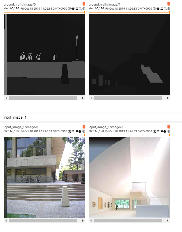
  tf.summary.image("input_image", image, max_outputs=2)
  tf.summary.image("ground_truth", tf.cast(annotation, tf.uint8), max_outputs=2)
  tf.summary.image("pred_annotation", tf.cast(pred_annotation, tf.uint8), max_outputs=2)

Loss, Optimization 선언, Tensorboard에 Loss기록

  # 손실함수를 선언하고 손실함수에 대한 summary를 지정합니다.
  loss = tf.reduce_mean((tf.nn.sparse_softmax_cross_entropy_with_logits(logits=logits,
                                                                        labels=tf.squeeze(annotation, squeeze_dims=[3]), name="entropy")))
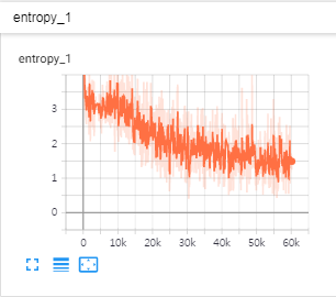
  tf.summary.scalar("entropy", loss)

  # 옵티마이저를 선언하고 파라미터를 한스텝 업데이트하는 train_step 연산을 정의합니다.
  optimizer = tf.train.AdamOptimizer(FLAGS.learning_rate)
  train_step = optimizer.minimize(loss)

Dataset을 불러오고 Batch단위로 묶는다.

 # training 데이터와 validation 데이터의 개수를 불러옵니다.
  print("Setting up image reader...")
  train_records, valid_records = scene_parsing.read_dataset(FLAGS.data_dir)
  print(len(train_records))
  print(len(valid_records))

  # training 데이터와 validation 데이터를 불러옵니다.
  print("Setting up dataset reader")
  image_options = {'resize': True, 'resize_size': IMAGE_SIZE}
  if FLAGS.mode == 'train':
    train_dataset_reader = dataset.BatchDatset(train_records, image_options)
  validation_dataset_reader = dataset.BatchDatset(valid_records, image_options)

Session을 열고 Train의 Log들을 지정한 Directory로 저장

  # 세션을 엽니다.
  sess = tf.Session()

  # 학습된 파라미터를 저장하기 위한 tf.train.Saver()와
  # tensorboard summary들을 저장하기 위한 tf.summary.FileWriter를 선언합니다.
  print("Setting up Saver...")
  saver = tf.train.Saver()
  summary_writer = tf.summary.FileWriter(FLAGS.logs_dir, sess.graph)

  # 변수들을 초기화하고 저장된 ckpt 파일이 있으면 저장된 파라미터를 불러옵니다.
  sess.run(tf.global_variables_initializer())
  ckpt = tf.train.get_checkpoint_state(FLAGS.logs_dir)
  if ckpt and ckpt.model_checkpoint_path:
    saver.restore(sess, ckpt.model_checkpoint_path)
    print("Model restored...")

선언한 Model과 Parameter를 통하여 학습을 진행
위에서 정의한 FLAG.mode에 따라서 Train을 할 것인지 결과를 저장하는 Visualisation을 할지 지정한다.

  if FLAGS.mode == "train":
    for itr in range(MAX_ITERATION):
      # 학습 데이터를 불러오고 feed_dict에 데이터를 지정합니다
      train_images, train_annotations = train_dataset_reader.next_batch(FLAGS.batch_size)
      feed_dict = {image: train_images, annotation: train_annotations, keep_probability: 0.85}

      # train_step을 실행해서 파라미터를 한 스텝 업데이트합니다.
      sess.run(train_step, feed_dict=feed_dict)

      # 10회 반복마다 training 데이터 손실 함수를 출력합니다.
      if itr % 10 == 0:
        train_loss, summary_str = sess.run([loss, summary_op], feed_dict=feed_dict)
        print("반복(Step): %d, Training 손실함수(Train_loss):%g" % (itr, train_loss))
        summary_writer.add_summary(summary_str, itr)

      # 500회 반복마다 validation 데이터 손실 함수를 출력하고 학습된 모델의 파라미터를 model.ckpt 파일로 저장합니다.
      if itr % 500 == 0:
        valid_images, valid_annotations = validation_dataset_reader.next_batch(FLAGS.batch_size)
        valid_loss = sess.run(loss, feed_dict={image: valid_images, annotation: valid_annotations,
                                               keep_probability: 1.0})
        print("%s ---> Validation 손실함수(Validation_loss): %g" % (datetime.datetime.now(), valid_loss))
        saver.save(sess, FLAGS.logs_dir + "model.ckpt", itr)

  elif FLAGS.mode == "visualize":
    # validation data로 prediction을 진행합니다.
    valid_images, valid_annotations = validation_dataset_reader.get_random_batch(FLAGS.batch_size)
    pred = sess.run(pred_annotation, feed_dict={image: valid_images, annotation: valid_annotations,
                                                keep_probability: 1.0})
    valid_annotations = np.squeeze(valid_annotations, axis=3)
    pred = np.squeeze(pred, axis=3)

    # Input Data, Ground Truth, Prediction Result를 저장합니다.
    for itr in range(FLAGS.batch_size):
      utils.save_image(valid_images[itr].astype(np.uint8), FLAGS.logs_dir, name="inp_" + str(5+itr))
      utils.save_image(valid_annotations[itr].astype(np.uint8), FLAGS.logs_dir, name="gt_" + str(5+itr))
      utils.save_image(pred[itr].astype(np.uint8), FLAGS.logs_dir, name="pred_" + str(5+itr))
      print("Saved image: %d" % itr)

  # 세션을 닫습니다.
  sess.close()

# main 함수를 실행합니다.
if __name__ == "__main__":
  tf.app.run()

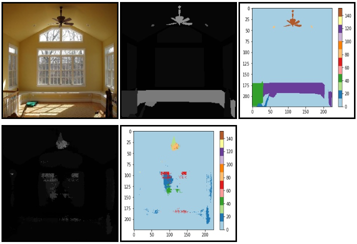
결과 확인

result_color_visualization.ipynb

Tensorboard1

Tensorboard2

---

참조:원본코드
참조: bskyvision.com
참조: shekkizh GitHub
참조: modulabs-biomedical 블로그
참조: ataspinar.com
참조:텐서플로로 배우는 딥러닝
문제가 있거나 궁금한 점이 있으면 wjddyd66@naver.com으로 Mail을 남겨주세요.