Tensorflow-CNN

CNN

CNN 은 딥러닝 이미지 처리 사용하는 인공신경망(Artificial Neural Network)이다.
CNN에 해당하는 이론에 대한 내용은 아래 링크를 참조하자.

1. CNN이란
2. CNN종류
3. CNN구현

위의 내용에서 이번 Post에서는 Tensorflow를 활용하여 CNN를 구현해보자

CNN Tnesorflow API

CNN을 Tensorflow에서 구현하기 전에 CNN에서 사용하는 Tensorflow API에 대해 먼저 알아보자.
1. Convolution
Convolution연산은 아래와 같은 Tensorflow API로서 진행된다.
Convolution Tensorflow API

tf.nn.conv2d( input, filter, strides, padding, dilations=[1,1,1,1], name=None )

• input: Input Data
• filter: Convolution 연산에 적용할 필터이며 [filter_height, filter_width, in_channels, out_channels] 형태의 4-D Tensor만 가능
• strides: 몇 Pixel 씩 넘어갈 지 지정
• padding
• ‘SAME’: zero padding 을 통하여 input 과 같은 크기의 이미지가 return
• ‘VALID’: Convolution 연산 공식에 의해 계산된 가로, 세로, 차원이 return
• dilation: Dilation Factor

2. Pooling
Pooling연산은 아래와 같은 Tensorflow API로서 진행된다.
Pooling Tensorflow API
Max Pooling

tf.nn.max_pool( value, ksize, strides, name=None )

• value: Max Pooling을 적용시킬 Input Data
• ksize: Max Pooling 연산에 적용할 필터이며 [batch_filter,height_filter, width_filter, channel_filter]형태의 4-D Tensor만 가능
• strides: 몇 Pixel씩 넘어갈지 지정

Mean Pooling

tf.nn.avg_pool;( value, ksize, strides, name=None )

• value: Max Pooling을 적용시킬 Input Data
• ksize: Max Pooling 연산에 적용할 필터이며 [batch_filter,height_filter, width_filter, channel_filter]형태의 4-D Tensor만 가능
• strides: 몇 Pixel씩 넘어갈지 지정

3. Dropout
Dropout연산은 아래와 같은 Tensorflow API로서 진행된다.
Dropout Tensorflow API

tf.nn.dropout( x, keep_prob, name=None )

• x: Dropout을 적용할 Input Data
• keep_prob: 드롭하지 않고 유지할 노드의 비율을 나타내는 scalar 텐서

CNN 실제 구현

텐퍼플로 라이브러리를 임포트

import tensorflow as tf

MNIST 데이터를 다운받고 불러오는 과정

from tensorflow.examples.tutorials.mnist import input_data
mnist = input_data.read_data_sets("/tmp/data/", one_hot=True)

CNN 모델을 정의

• Convolution Layer: 2개
• Pooling Layer: 2개

x_image = tf.reshape(x,[-1,28,28,1])에서 -1으 data의 dimension을 모를 때 유용하게 사용할 수 있다.

row 또는 Column중 하나만 값을 정해주고 나머지에 -1을 넣어준다면, 정해준 값에 맞춰서 reshape가 이루어 진다.

즉 우리는 batch를 통하여 Trainning 을 하기 때문에 -1을 넣어주어서 batch size에 맞게 dynamic 한 input 행렬을 만들어야 하므로 [-1, 28, 28, 1]로서 정의한 것이다.

또한 현재 MNIST 의 Image는 흑백으로서 Channel의 개수가 정의되어 있지 않으므로 뒤에 1로서 Channel을 직접 정의해야 하는 상황이다.

#CNN Model Definition
def build_CNN_Classifier(x):
    #MNIST 데이터를 3차원 형태로 reshape(흑백이므로 채널은 1)
    x_image = tf.reshape(x,[-1,28,28,1])
    
    # 1_Convolution_Layer
    # 5 x 5 Filter 32개 적용
    # 28 x 28 => 28 x 28 x 32
    W_conv1 = tf.Variable(tf.truncated_normal(shape=[5,5,1,32],stddev=5e-2))
    #truncated: 정규 분포로서 출력
    b_conv1 = tf.Variable(tf.constant(0.1, shape=[32]))
    h_conv1 = tf.nn.relu(tf.nn.conv2d(x_image, W_conv1, strides=[1,1,1,1],padding='SAME')+b_conv1)
    
    # 1_Pooling Layer
    # Max_Pooling => Image size 1/2
    # 28 x 28 x 32 => 14 x 14 x 32
    h_pool1 = tf.nn.max_pool(h_conv1,ksize=[1,2,2,1],strides=[1,2,2,1],padding='SAME')
    
    # 2_Convolution_Layer
    # 5 x 5 Filter 64개 적용
    # 14 x 14 x 32 => 14 x 14 x 64
    W_conv2 = tf.Variable(tf.truncated_normal(shape=[5,5,32,64],stddev=5e-2))
    #truncated: 정규 분포로서 출력
    b_conv2 = tf.Variable(tf.constant(0.1, shape=[64]))
    h_conv2 = tf.nn.relu(tf.nn.conv2d(h_pool1, W_conv2,strides=[1,1,1,1],padding='SAME')+b_conv2)
    
    # 2_Pooling Layer
    # Max_Pooling => Image size 1/2
    # 14 x 14 x 64 => 7 x 7 x 64
    h_pool2 = tf.nn.max_pool(h_conv2,ksize=[1,2,2,1],strides=[1,2,2,1],padding='SAME')
    
    # 완전 연결층
    # 7 x 7 크기를 가진 64개의 activation map을 1024개의 특징들로 변환
    # 7 x 7 x 64(3136) => 1024
    W_fc1 = tf.Variable(tf.truncated_normal(shape=[7*7*64, 1024],stddev=5e-2))
    b_fc1 = tf.Variable(tf.constant(0.1,shape=[1024]))
    h_pool2_flat = tf.reshape(h_pool2,[-1,7*7*64])
    h_fc1 = tf.nn.relu(tf.matmul(h_pool2_flat,W_fc1)+b_fc1)
    
    # 출력층
    # 1024개의 특징들(feature)을 10개의 class로 변환
    # 1024 -> 10
    W_output = tf.Variable(tf.truncated_normal(shape=[1024,10],stddev=5e-2))
    b_output = tf.Variable(tf.constant(0.1,shape=[10]))
    logits = tf.matmul(h_fc1,W_output)+b_output
    y_pred = tf.nn.softmax(logits)
    
    return y_pred, logits

Input 과 Output 데이터를 받을 Place Holder 정의

x = tf.placeholder(tf.float32, shape=[None, 784])
y = tf.placeholder(tf.float32, shape=[None, 10])

Model 생성

y_pred, logits = build_CNN_Classifier(x)

• LosttFunction: Cross_Entropy_with_Softmax
• Optimzer: Adam

loss = tf.reduce_mean(tf.nn.softmax_cross_entropy_with_logits(labels=y, logits=logits))
train_step = tf.train.AdamOptimizer(1e-04).minimize(loss)

정확도를 출력하기 위한 연산들을 정의

correct_prediction = tf.equal(tf.argmax(y_pred,1),tf.argmax(y,1))
accuracy = tf.reduce_mean(tf.cast(correct_prediction, tf.float32))

Session을 열고 그래프 실행하여 학습 실행

with tf.Session() as sess:
    #모든 변수 초기화
    sess.run(tf.global_variables_initializer())
    
    for i in range(3000):
        #50개씩 MNIST 데이터를 불러온다.
        batch = mnist.train.next_batch(50)
        
        if i % 100 ==0:
            train_accuracy = accuracy.eval(feed_dict={x:batch[0], y:batch[1]})
            print('반복(Epoch): %d, 정확도: %f'%(i, train_accuracy))
            
        sess.run([train_step], feed_dict={x:batch[0], y: batch[1]})
        
    #정확도 측정
    print('Model 정확도: %f'%accuracy.eval(feed_dict={x:mnist.test.images, y: mnist.test.labels}))

반복(Epoch): 0, 정확도: 0.160000
반복(Epoch): 100, 정확도: 0.740000
반복(Epoch): 200, 정확도: 0.880000

...

반복(Epoch): 2500, 정확도: 0.980000
반복(Epoch): 2600, 정확도: 0.980000
반복(Epoch): 2700, 정확도: 1.000000
반복(Epoch): 2800, 정확도: 0.980000
반복(Epoch): 2900, 정확도: 0.980000

결과
Model 정확도: 0.983400

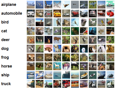
CNN 을 이용한 CIFAR-10 이미지 분류기

CIFAR-10은 총 10개의 레이블로 구성된 이미지 분류를 위한 Dataset이다.
Image는 32 x 32의 크기의 이미지로 되어있고 또한 MNIST와 달리 Color Image인 것이 특징이다.
아래 사진은 CIFAR-10의 Dataset의 일부이다.

CNN 을 이용한 CIFAR-10 이미지 분류기 구현

numpy 라이브러리 import
CIFAR-10 데이터셋을 다운받고, 불러오는 과정을 지원하는 helper 함수를 keras 모듈에서 load_data라는 모듈 함수로 제공

import numpy as np
from tensorflow.keras.datasets.cifar10 import load_data

데이터를 배치 개수만큼 끊어서 읽어올 수 있는 next_batch 함수 선언

def next_batch(num, data, labels):
    idx = np.arange(0, len(data))
    np.random.shuffle(idx)
    idx = idx[:num]
    data_shuffle = [data[i] for i in idx]
    labels_shuffle = [labels[i] for i in idx]
    
    return np.asarray(data_shuffle), np.asarray(labels_shuffle)

CNN 모델을 정의

• Convolution Layer: 5개
• Pooling Layer: 2개
• DropOut Layer: 1개

#CNN Model Definition
def build_CNN_Classifier(x):
    x_image = x
    
    # 1_Convolution_Layer
    # RGB(Color) image를 64개의 feature으로 mapping 과정
    W_conv1 = tf.Variable(tf.truncated_normal(shape=[5,5,3,64],stddev=5e-2))
    #truncated: 정규 분포로서 출력
    b_conv1 = tf.Variable(tf.constant(0.1, shape=[64]))
    h_conv1 = tf.nn.relu(tf.nn.conv2d(x_image, W_conv1, strides=[1,1,1,1],padding='SAME')+b_conv1)
    
    # 1_Pooling Layer
    h_pool1 = tf.nn.max_pool(h_conv1,ksize=[1,3,3,1],strides=[1,2,2,1],padding='SAME')
    
    # 2_Convolution_Layer
    # 64개의 feature을 다시 64개의 feature으로 mapping 하는 과정
    W_conv2 = tf.Variable(tf.truncated_normal(shape=[5,5,64,64],stddev=5e-2))
    #truncated: 정규 분포로서 출력
    b_conv2 = tf.Variable(tf.constant(0.1, shape=[64]))
    h_conv2 = tf.nn.relu(tf.nn.conv2d(h_pool1, W_conv2,strides=[1,1,1,1],padding='SAME')+b_conv2)
    
    # 2_Pooling Layer
    h_pool2 = tf.nn.max_pool(h_conv2,ksize=[1,3,3,1],strides=[1,2,2,1],padding='SAME')
    
    # 3_Convolution_Layer
    # 64개의 feature을 다시 128개의 feature으로 mapping 하는 과정
    W_conv3 = tf.Variable(tf.truncated_normal(shape=[3,3,64,128],stddev=5e-2))
    #truncated: 정규 분포로서 출력
    b_conv3 = tf.Variable(tf.constant(0.1, shape=[128]))
    h_conv3 = tf.nn.relu(tf.nn.conv2d(h_pool2, W_conv3,strides=[1,1,1,1],padding='SAME')+b_conv3)
    
    
    # 4_Convolution_Layer
    # 128개의 feature을 다시 128개의 feature으로 mapping 하는 과정
    W_conv4 = tf.Variable(tf.truncated_normal(shape=[3,3,128,128],stddev=5e-2))
    #truncated: 정규 분포로서 출력
    b_conv4 = tf.Variable(tf.constant(0.1, shape=[128]))
    h_conv4 = tf.nn.relu(tf.nn.conv2d(h_conv3, W_conv4,strides=[1,1,1,1],padding='SAME')+b_conv4)
    
    
    # 5_Convolution_Layer
    # 128개의 feature을 다시 128개의 feature으로 mapping 하는 과정
    W_conv5 = tf.Variable(tf.truncated_normal(shape=[3,3,128,128],stddev=5e-2))
    #truncated: 정규 분포로서 출력
    b_conv5 = tf.Variable(tf.constant(0.1, shape=[128]))
    h_conv5 = tf.nn.relu(tf.nn.conv2d(h_conv4, W_conv5,strides=[1,1,1,1],padding='SAME')+b_conv5)
    
    # 완전 연결층
    # 2번의 downsampling 이후에, 32 x 32 이미지는 8 x 8 x 128의 Feature map으로 변환
    W_fc1 = tf.Variable(tf.truncated_normal(shape=[8*8*128, 384],stddev=5e-2))
    b_fc1 = tf.Variable(tf.constant(0.1,shape=[384]))
    h_conv5_flat = tf.reshape(h_conv5,[-1,8*8*128])
    h_fc1 = tf.nn.relu(tf.matmul(h_conv5_flat,W_fc1)+b_fc1)
    
    # Dropout - 모델의 복잡도를 컨트롤
    # 특징들의 co-adaptation을 방지
    h_fc1_drop = tf.nn.dropout(h_fc1, keep_prob)
    
    # 완전 연결층2
    # 384개의 feature를 10개의 class로 Mapping
    W_fc2 = tf.Variable(tf.truncated_normal(shape=[384, 10],stddev=5e-2))
    b_fc2 = tf.Variable(tf.constant(0.1,shape=[10]))
    logits = tf.matmul(h_fc1_drop, W_fc2) + b_fc2
    y_pred = tf.nn.softmax(logits)
    
    return y_pred, logits

• x: Input Data
• y: OutputData
• keep_prob= 드롭아웃에서 드롭하지 않고 유지할 노드 비율

x = tf.placeholder(tf.float32, shape = [None, 32, 32, 3])
y = tf.placeholder(tf.float32, shape = [None, 10])
keep_prob = tf.placeholder(tf.float32)

load_data()함수를 이용하여 CIFAR-10 데이터를 다운로드하고 tf.one_hot API 를 이용해서 스칼라값 형태의 레이블 (0~9)을 One-hot-Encoding 형태로 변환
squeeze: Removes dimensions of size 1 from the shape of a tensor

(x_train, y_train), (x_test, y_test) = load_data()
#Scalar 현태의 0 ~ 9 형태의 0 ~ 9 을 One - hot Encoding 형태로 변환
y_train_one_hot = tf.squeeze(tf.one_hot(y_train,10),axis=1)
y_test_one_hot = tf.squeeze(tf.one_hot(y_test,10),axis=1)

Model 생성

• LosttFunction: Cross Entropy
• Optimzer: RMSPropr

y_pred, logits = build_CNN_Classifier(x)

loss = tf.reduce_mean(tf.nn.softmax_cross_entropy_with_logits(labels=y,logits=logits))
train_step = tf.train.RMSPropOptimizer(1e-3).minimize(loss)

정확도를 출력하기 위한 연산들을 정의

correct_prediction = tf.equal(tf.argmax(y_pred,1),tf.argmax(y,1))
accuracy = tf.reduce_mean(tf.cast(correct_prediction,tf.float32))

Session을 열고 그래프 실행하여 학습 실행

with tf.Session() as sess:
    #모든 변수를 초기화
    sess.run(tf.global_variables_initializer())
    
    for i in range(10000):
        batch = next_batch(128, x_train, y_train_one_hot.eval())
        
        if i % 100 == 0:
            train_accuracy = accuracy.eval(feed_dict={x: batch[0], y: batch[1], keep_prob: 1.0})
            loss_print = loss.eval(feed_dict={x: batch[0], y: batch[1], keep_prob: 1.0})
            
            print('반복(Epoch): %d, 정확도: %f, 손실함수: %f'%(i, train_accuracy, loss_print))
            
            #20 % Dropout을 활용하여 학습을 진행
        sess.run(train_step, feed_dict={x: batch[0], y:batch[1], keep_prob:0.8})
            
    #학습이 끝나면 테스트 데이터에 대한 정확도를 출력
    test_accuracy = 0.0
    for i in range(10):
        test_batch = next_batch(1000,x_test,y_test_one_hot.eval())
        test_accuracy = test_accuracy + accuracy.eval(feed_dict={x: test_batch[0], y:test_batch[1], keep_prob: 1.0})
            
    test_accuracy = test_accuracy/10
    print('테스트 데이터 정확도: %f'%(test_accuracy))

반복(Epoch): 0, 정확도: 0.109375, 손실함수: 101.231110
반복(Epoch): 100, 정확도: 0.148438, 손실함수: 2.251683
반복(Epoch): 200, 정확도: 0.296875, 손실함수: 2.232113

...

반복(Epoch): 9700, 정확도: 0.695312, 손실함수: 0.826372
반복(Epoch): 9800, 정확도: 0.710938, 손실함수: 0.783436
반복(Epoch): 9900, 정확도: 0.609375, 손실함수: 1.050041

결과
테스트 데이터 정확도: 0.642000

tf.train.Saver API

tf.train.Saver API 란 모델과 파라미터를 저장하고 불러오는 방법이다.
딥러닝 기법을 이용해서 복잡한 문제를 해결할 때는 수많은 횟수를 반복해서 파라미터를 업데이트 해야 하나 매번 바닥부터 파라미터를 새로 업데이트하는 것은 비효율적이므로 학습한 모델의 파라미터를 저장하고 불러오는 방법을 사용한다.
tf.train.Saver() 클래스를 선언
선언한 tf.train.Saver()클래스의 save(sess, save_path, global_step=None)함수를 호출해서 모델과 파라미터를 저장한다.

1. save_path: 모델과 파라미터를 저장할 폴더경로 + 저장할 이름
2. global_step: 반복회수
3. restore(sess, save_path): 저장된 모델과 파라미터를 불러오는 방법

위에 선언된 CNN 모델을 이용한 MNIST 숫자 분류기 코드에 tf.train.Saver API 를 이용해서 학습한 모델의 파라미터를 저장하고 불러오는 방법 사용
Model 정의

#CNN Model Definition
def build_CNN_Classifier(x):
    #MNIST 데이터를 3차원 형태로 reshape(흑백이므로 채널은 1)
    x_image = tf.reshape(x,[-1,28,28,1])
    
    # 1_Convolution_Layer
    # RGB(Color) image를 64개의 feature으로 mapping 과정
    W_conv1 = tf.Variable(tf.truncated_normal(shape=[5,5,1,32],stddev=5e-2))
    #truncated: 정규 분포로서 출력
    b_conv1 = tf.Variable(tf.constant(0.1, shape=[32]))
    h_conv1 = tf.nn.relu(tf.nn.conv2d(x_image, W_conv1, strides=[1,1,1,1],padding='SAME')+b_conv1)
    
    # 1_Pooling Layer
    h_pool1 = tf.nn.max_pool(h_conv1,ksize=[1,2,2,1],strides=[1,2,2,1],padding='SAME')
    
    # 2_Convolution_Layer
    # 64개의 feature을 다시 64개의 feature으로 mapping 하는 과정
    W_conv2 = tf.Variable(tf.truncated_normal(shape=[5,5,32,64],stddev=5e-2))
    #truncated: 정규 분포로서 출력
    b_conv2 = tf.Variable(tf.constant(0.1, shape=[64]))
    h_conv2 = tf.nn.relu(tf.nn.conv2d(h_pool1, W_conv2,strides=[1,1,1,1],padding='SAME')+b_conv2)
    
    # 2_Pooling Layer
    h_pool2 = tf.nn.max_pool(h_conv2,ksize=[1,2,2,1],strides=[1,2,2,1],padding='SAME')
        
    # 완전 연결층
    W_fc1 = tf.Variable(tf.truncated_normal(shape=[7*7*64, 1024],stddev=5e-2))
    b_fc1 = tf.Variable(tf.constant(0.1,shape=[1024]))
    h_pool2_flat = tf.reshape(h_pool2,[-1,7*7*64])
    h_fc1 = tf.nn.relu(tf.matmul(h_pool2_flat,W_fc1)+b_fc1)
    
    #출력층
    W_output = tf.Variable(tf.truncated_normal(shape=[1024,10],stddev=5e-2))
    b_output = tf.Variable(tf.constant(0.1,shape=[10]))
    logits = tf.matmul(h_fc1,W_output)+b_output
    y_pred = tf.nn.softmax(logits)
    
    return y_pred, logits

인풋, 아웃풋 데이터를 받기위한 플레이스 홀더를 정의

x = tf.placeholder(tf.float32, shape=[None, 784])
y = tf.placeholder(tf.float32, shape=[None, 10])

Model 생성

y_pred, logits = build_CNN_Classifier(x)

• LosttFunction: Cross_Entropy_with_Softmax
• Optimzer: Adam

loss = tf.reduce_mean(tf.nn.softmax_cross_entropy_with_logits(labels=y, logits=logits))
train_step = tf.train.AdamOptimizer(1e-04).minimize(loss)

정확도를 출력하기 위한 연산들을 정의

correct_prediction = tf.equal(tf.argmax(y_pred,1),tf.argmax(y,1))
accuracy = tf.reduce_mean(tf.cast(correct_prediction, tf.float32))

tf.train.Saver를 이용해서 모델과 파라미터를 저장

import os

SAVE_DIR = 'model'
saver = tf.train.Saver()
chekpoint_path = os.path.join(SAVE_DIR, 'model')
ckpt = tf.train.get_checkpoint_state(SAVE_DIR)

Session을 열고 그래프 실행하여 학습 실행
만약 저장된 모델과 파라미터가 있으면 이를 불러오고(Restore)
Restored 모델을 이용해서 테스트 데이터에 대한 정확도를 출력하고 프로그램을 종료

with tf.Session() as sess:
    #모든 변수 초기화
    sess.run(tf.global_variables_initializer())
    
    #만약 저장된 모델과 파라미터가 있으면 이를 불러오고(Restore)
    #Restored 모델을 이용해서 테스트 데이터에 대한 정확도를 출력하고 프로그램을 종료
    if ckpt and ckpt.model_checkpoint_path:
        saver.restore(sess,ckpt.model_checkpoint_path)
        print('테스트 데이터 정확도(Restored): %f'%accuracy.eval(feed_dict={x: mnist.test.images, y:mnist.test.labels}))
        sess.close()
        exit()
    
    for i in range(3000):
        #50개씩 MNIST 데이터를 불러온다.
        batch = mnist.train.next_batch(50)
        
        if i % 100 ==0:
            saver.save(sess,chekpoint_path,global_step=i)
            train_accuracy = accuracy.eval(feed_dict={x:batch[0], y:batch[1]})
            print('반복(Epoch): %d, 정확도: %f'%(i, train_accuracy))
            
        sess.run([train_step], feed_dict={x:batch[0], y: batch[1]})
        
    #정확도 측정
    print('Model 정확도: %f'%accuracy.eval(feed_dict={x:mnist.test.images, y: mnist.test.labels}))

반복(Epoch): 0, 정확도: 0.100000
반복(Epoch): 100, 정확도: 0.860000
반복(Epoch): 200, 정확도: 0.880000

...

반복(Epoch): 2700, 정확도: 0.960000
반복(Epoch): 2800, 정확도: 1.000000
반복(Epoch): 2900, 정확도: 0.980000

결과
Model 정확도: 0.984500

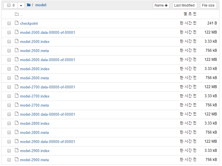
이렇게 저장된 File은 Checkpoint State Protocol Buffer이다.
이러한 Protocol Buffer에 관한 자세한 내용은 아래 링크 참조
Protocol Buffer 자세한 내용

---

참조:원본코드
참조:텐서플로로 배우는 딥러닝
문제가 있거나 궁금한 점이 있으면 wjddyd66@naver.com으로 Mail을 남겨주세요.